Trending Topics and Top-K
A system design interview guide to finding the most frequent items in a massive stream — trending hashtags, top products, hottest search terms — when the universe of items is too large to count exactly and "trending" means recency, not all-time totals.
"Show me the top ten trending hashtags" is a question every social product answers, and it hides a genuinely hard counting problem. The stream of items is unbounded and the set of distinct items — hashtags, product ids, search queries — runs into the millions or more, most of them rare. Keeping an exact counter for every item so you can sort and take the top k means a hash map the size of the entire item universe, updated on every event. The way out is to give up exactness for the long tail you do not care about while staying accurate for the heavy hitters you do, using a probabilistic frequency sketch paired with a small heap. This guide builds that design up, then extends it to the recency that makes a count "trending" and to merging results across shards.
Contents
1. The Top-K Problem
The Top-K problem is: given a stream of items where the same item appears many times, report the k items with the highest frequency. It sounds like a sorting problem, but the scale changes its character — you cannot afford to keep an exact, sorted tally of a stream that never ends over a universe of items that is enormous and mostly irrelevant.
The applications are the recommendation and discovery surfaces of almost any product:
- Trending hashtags or topics — the tags appearing far more than usual right now, surfaced on a discovery page.
- Top products — the most-viewed or most-purchased items, for a "popular now" rail or merchandising.
- Hottest search queries — the queries spiking in volume, for autosuggest and editorial surfacing.
What makes this its own design topic, distinct from plain distinct-counting, is the shape of the data. Item frequencies follow a heavy-tailed distribution: a handful of items are wildly popular and the overwhelming majority appear only a few times. You only ever care about the head of that distribution — the top k — yet an exact approach is forced to spend memory tracking the entire tail just in case. The whole game is to be accurate about the heavy hitters while refusing to pay for the millions of items that will never come close to the top.
2. Why Exact Top-K Is Expensive
The exact solution is a hash map from item to count, incremented on every event, with the top k read off by sorting (or maintaining a heap). It is correct, and at small scale it is fine. The cost problem is the size of the map, and it is driven by the long tail rather than the heavy hitters.
Because the map needs an entry for every distinct item that has ever appeared, its memory scales with the size of the item universe, not with k. In a heavy-tailed stream the universe is dominated by rare items — millions of hashtags used once or twice — and you are paying to store a counter for every single one of them, even though none will ever be in the top ten. You are spending almost all of your memory on items the answer will never mention.
At stream scale this map becomes too large to hold in memory on one machine, which forces it into a distributed store and turns every increment into a network operation against hot keys. The exact approach is not wrong; it simply ties memory to the wrong quantity — the breadth of the tail — when the question only concerns the head.
The escape, as with distinct counting, is a tolerance the consumer already has: a trending list does not need exact counts, only the right items in roughly the right order. If item frequencies are estimated with a small, bounded error, the ranking of the heavy hitters is preserved, and the rare items can be allowed to collide and share space because their exact counts never mattered. That tolerance is what the Count-Min Sketch exploits.
3. Count-Min Sketch
A Count-Min Sketch (CMS) is a compact, fixed-size structure that estimates how many times each item has been seen, using far less memory than an exact map by deliberately letting different items share counters. It is the frequency analogue of the bit tricks behind cardinality sketches: trade a little accuracy for a memory footprint that does not grow with the item universe.
Structurally a CMS is a two-dimensional array of counters: d rows and w columns, with one independent hash function per row. To record an item, you hash it once per row to pick one column in that row and increment all d of those counters. Different items may hash to the same column in some row — a collision — and when they do they share that counter, which is the source of both the memory savings and the error.
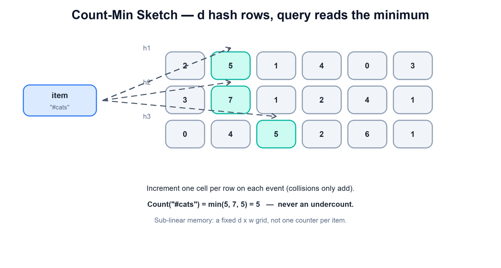
The clever part is the query. To estimate an item's count you look at its d chosen counters — one per row — and take the minimum. Every one of those counters includes the item's true count plus whatever other items happened to collide with it in that cell, so each counter is an overestimate. The minimum is the least-contaminated of them, the cell where the fewest other items landed. This gives a one-sided guarantee that is exactly what Top-K needs: the estimate is never below the true count, and only ever an overestimate, with the overshoot bounded by the sketch's dimensions.
# increment: one cell per row, all d rows
function cms_add(cms, item, count=1):
  for r in range(d):
    c = hash[r](item) % w          # this row's column for the item
    cms[r][c] += count             # shared cell — collisions just add

# query: minimum over the d cells is the least-contaminated estimate
function cms_estimate(cms, item):
  return min(cms[r][hash[r](item) % w] for r in range(d))   # never an undercount
The memory win is that the grid is a fixed d × w size chosen for the accuracy you want, completely independent of how many distinct items the stream contains. Adding a millionth rare hashtag costs nothing — it just collides into existing cells — whereas the exact map would allocate a new entry. The structure is sub-linear in the item universe by construction.
4. Pairing CMS with a Heap
A CMS estimates the frequency of any item you ask about, but on its own it cannot tell you which items are the top k — it has thrown away the identities. To produce the actual list you pair the sketch with a small min-heap of size k that remembers the current leading items and their estimated counts.
The heap holds at most k entries and is ordered so that its root is the smallest estimate among the current leaders — the weakest member of the top k, and therefore the one most easily displaced. This is the standard structure for "keep the largest k things seen so far," and keeping it at exactly size k means it costs a tiny, fixed amount of memory regardless of stream length or item universe.
The two structures divide the labour cleanly. The CMS answers "how often has this item been seen?" in fixed memory; the heap answers "is that frequent enough to be in the current top k, and if so who does it bump?" Neither could do the job alone: the sketch lacks identities, and a heap over raw counts would need the exact per-item tallies the sketch is there to avoid.
5. The Streaming Algorithm
With both structures in hand, processing each event is a short, constant-time routine. The sketch is updated, the item's fresh estimate is read back, and that estimate is checked against the weakest current leader to decide whether the heap changes.
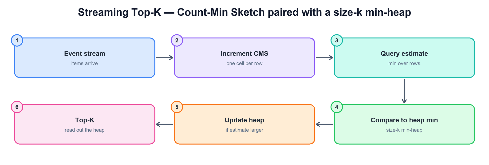
The per-event logic, step by step:
- Increment the sketch. Add the item to the CMS, bumping one counter in each of the d rows.
- Query the estimate. Read the item's current estimated count back from the sketch as the minimum over its rows.
- Compare to the heap. If the item is already in the heap, refresh its stored estimate (and re-heapify). Otherwise compare its estimate to the heap's minimum — the weakest leader. If the estimate is larger and the heap is full, evict the root and insert this item; if the heap is not yet full, just insert.
function on_item(cms, heap, item):
  cms_add(cms, item)                        # d increments
  est = cms_estimate(cms, item)             # min over rows
  if heap.contains(item):
    heap.update(item, est)                  # already a leader; refresh
  elif len(heap) < K:
    heap.push(item, est)                    # room to spare
  elif est > heap.peek_min():               # beats the weakest leader?
    heap.pop_min()                          # evict the weakest
    heap.push(item, est)                    # promote this item

function top_k(heap):
  return heap.sorted_desc()                 # read out the current top-k
Every step is O(d) for the sketch plus O(log k) for the heap — constant with respect to the stream length and the item universe. Memory is the fixed CMS grid plus k heap entries. That bounded, per-event cost is exactly what an unbounded stream demands.
6. Sliding and Decaying Windows
So far the counts are all-time totals, which gives "most popular ever," not "trending." Trending is about recency: an item that is spiking now should rank above one that was huge last year and is now quiet. To capture that, the counting has to forget the past, which means adding a notion of a time window.
Two common approaches express recency:
- Sliding / tumbling windows. Maintain separate sketches per time bucket — one per minute or per hour — and compute trending over only the recent buckets, discarding old ones as they age out. A bucket that falls outside the window is simply dropped, so its counts stop contributing. This gives a crisp "last N minutes" view at the cost of keeping several sketches around.
- Decaying counts. Apply exponential decay so older observations contribute progressively less, either by periodically scaling all counters down by a factor or by weighting increments by recency. A single sketch then reflects a smoothly fading memory of the past, where recent activity dominates without a hard cutoff.
A frequent refinement is to define trending as a change in rate rather than raw recent frequency — comparing an item's count in the current window against its typical or previous-window count, so a perennially popular item is not always "trending" and a genuine surge stands out. The windowing machinery is the same; only the ranking signal changes from "how frequent" to "how much more frequent than usual."
7. Merging Across Shards
At scale the stream is partitioned across many machines, each maintaining its own CMS and heap over the slice of events it sees. Producing a single global Top-K means combining these per-shard results — and this is where Top-K differs sharply from cardinality sketches, because the merge is only approximate.
The Count-Min Sketches themselves merge cleanly: same dimensions and hash functions, add the grids cell by cell, and you get a sketch representing the union of all shards' events. The difficulty is the heaps. Each shard's heap only ever tracked the items that were heavy on that shard, so an item that was, say, the eleventh most popular on every shard — never quite making any local top ten — may be genuinely top ten globally yet appear in no shard's heap. Its identity was discarded locally before the merge could see it.
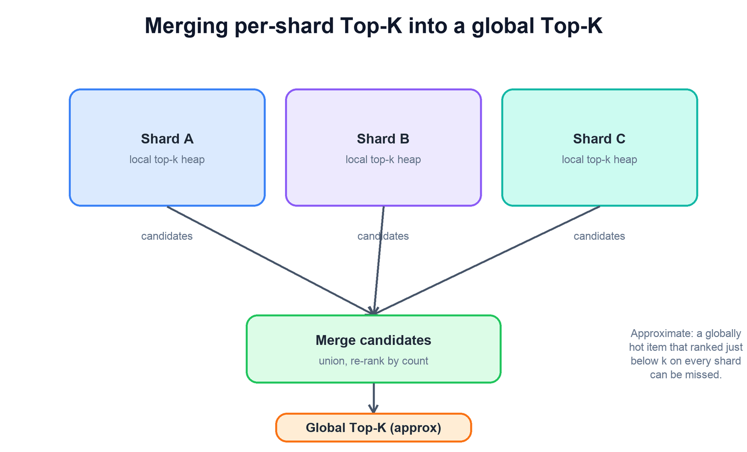
The practical merge therefore works on candidate sets: take the union of every shard's local top-k items, then re-rank that combined candidate list by global frequency — either by summing each candidate's per-shard estimates or by querying a merged sketch. To reduce the miss-an-item risk, shards usually track more than k locally (a top-2k or top-10k buffer), so an item that is moderately strong everywhere is more likely to survive into some shard's candidate list and reach the merge.
function global_top_k(shards, K):
  candidates = union(s.heap.items() for s in shards)   # local leaders only
  merged_cms = reduce(cms_merge, [s.cms for s in shards])
  scored = [(item, cms_estimate(merged_cms, item)) for item in candidates]
  return top_k_by_count(scored, K)                     # approximate — tail items can be missed
8. Accuracy Tradeoffs
The errors in a Top-K system come from two distinct places, and it helps to keep them separate when reasoning about accuracy.
- Sketch error (the counts). The CMS only ever overestimates, and the size of the overshoot shrinks as the grid grows. Roughly, the width w controls how large an overcount can be and the depth d controls how often the bound holds — wider rows mean fewer collisions per cell, more rows mean the minimum is more likely to find a clean one. You spend memory to tighten both.
- Merge error (the membership). Combining per-shard top-k lists can miss an item that was globally heavy but locally always just short of the cut. This is mitigated, not eliminated, by tracking more than k per shard.
| Knob / effect | What it controls |
|---|---|
| Width w (columns) | The magnitude of overcounting — wider rows spread items out, so each cell collects fewer foreign items. |
| Depth d (rows) | The confidence of the estimate — more independent hashes make it likelier the minimum cell is uncontaminated. |
| One-sided error | CMS never undercounts, so a true heavy hitter is never wrongly pushed out of the top-k by underestimation. |
| Local buffer > k | Tracking top-2k or more per shard reduces the chance of dropping a globally hot, locally-marginal item before the merge. |
| Heavy-tail friendliness | Errors land hardest on rare items (which you do not care about) and barely touch heavy hitters (which you do). |
The reason the whole approach works is that the errors fall where it is cheap to be wrong. Collisions inflate the counts of rare items the most, because heavy hitters dominate whichever cells they land in; the items at the top — the only ones the answer reports — are the most accurately estimated. You are approximate precisely about the tail you were going to ignore anyway.
9. Summary
A trending Top-K system finds the heaviest items in an unbounded stream without paying for the long tail. The design is a few interlocking decisions:
| Concern | Mechanism |
|---|---|
| What are we computing? | The k most frequent items in a stream — trending hashtags, top products, hottest queries. |
| Why not an exact counter map? | It needs an entry per distinct item, so memory scales with the (mostly irrelevant) item universe, not with k. |
| How do we estimate counts cheaply? | Count-Min Sketch: a d×w counter grid, increment one cell per row, query the minimum — a bounded overestimate in fixed memory. |
| How do we get the actual top-k items? | Pair the sketch with a size-k min-heap that tracks the current leaders by estimated count. |
| How does each event flow? | Increment the CMS, read the estimate, compare to the heap minimum, update the heap if it beats the weakest leader. |
| How do we make it "trending"? | Sliding/tumbling windows or decaying counts so recent activity outranks stale all-time totals. |
| How do we go global across shards? | Merge the sketches cell-wise and union the per-shard candidate lists, then re-rank — an approximate merge. |
| How accurate is it? | CMS only overcounts and is tunable via d and w; errors concentrate on the rare tail, leaving heavy hitters accurate. |