Designing a Metrics / Time-Series Store
A system design interview guide to building an operational metrics store — the kind that ingests millions of data points per second, keeps years of history without going broke, and answers a dashboard query in milliseconds.
Every large system is wired with sensors: counters for requests served, gauges for memory used, timers for latency, one metric for almost everything an operator might want to graph. Collected together at scale, these emit an astonishing firehose of timestamped numbers, and somebody has to store them in a way that is cheap to write, cheap to keep, and fast to query. A general-purpose database struggles with this workload because it was not built for it — the access pattern is overwhelmingly append-only writes and range-scan reads over a very specific shape of data. A purpose-built time-series store, of the sort an operational data store like ODS provides, makes a handful of specialized choices that a relational database cannot. This guide builds up those choices: the data model, the write path, downsampling into retention tiers, the compression tricks that make years of history affordable, and the query path that ties it together.
Contents
1. The Data Model
The whole design rests on a deliberately narrow data model. A single data point is the combination of four things, and pinning them down early is what lets every later layer be specialized.
- Metric name. What is being measured, for example
http.requestsorcpu.usage. It names the series family. - Tags / labels. A set of key-value pairs that identify which instance of that metric, for example
host=web42,region=us-east,status=200. The metric name plus its full set of tags defines a single, distinct time series. - Timestamp. When the measurement was taken, usually at second or millisecond resolution.
- Value. The number itself — a floating-point reading.
So a data point is (name, {tags}, timestamp, value), and a series is the ordered sequence of (timestamp, value) pairs that share one name-and-tags identity. This is the unit everything operates on: writes append a point to a series, reads scan a range within one or more series, and compression works down the (timestamp, value) columns of a series. The narrowness is the point — because the shape is so constrained, the storage engine can make assumptions a general database never could.
| Component | Example | Role |
|---|---|---|
| Metric name | http.requests | Names the family of series. |
| Tags | host=web42, status=200 | Selects one specific series within the family. |
| Timestamp | 1700000000 | Position along the time axis of that series. |
| Value | 97.3 | The measurement at that instant. |
2. Counters vs Gauges
Values come in two flavors, and the distinction changes how they are queried even though they are stored the same way. Knowing which is which is the difference between a sensible graph and a meaningless one.
- Gauges. A gauge is a snapshot reading that can go up or down — current memory in use, temperature, queue depth, number of active connections. You graph a gauge directly; its instantaneous value is meaningful on its own.
- Counters. A counter only ever increases — total requests served, total bytes sent, total errors since the process started. The raw value of a counter is almost never interesting; what you want is its rate of change. You graph a counter by taking the difference between consecutive points and dividing by the time between them, turning "total requests" into "requests per second."
3. High Cardinality
The hardest scaling problem in a metrics store is not the volume of points; it is the number of distinct series, known as cardinality. Cardinality is the product of every tag's distinct values. One metric tagged by host, status code, endpoint, and region explodes combinatorially: a thousand hosts times a hundred endpoints times a dozen status codes is already over a million distinct series from a single metric name.
Cardinality hurts because the store must track an index entry and an in-flight write buffer for every active series. A tag whose values are effectively unbounded — a user id, a request id, a raw timestamp jammed into a label — is the classic cardinality bomb: each new value mints a brand-new series forever, and the index grows without limit until memory is exhausted. The defenses are mostly disciplinary: keep tags to bounded, low-cardinality dimensions; never put unbounded identifiers in labels; and put limits and monitoring on series creation so a misbehaving client cannot take the system down by inventing millions of series.
| Tag | Cardinality | Verdict |
|---|---|---|
region | ~10 values | Fine — bounded and small. |
status | ~40 values | Fine — bounded. |
host | thousands | Acceptable, watch it. |
user_id | millions+ | Cardinality bomb — never use as a tag. |
4. The Write Path
The write path is engineered around one fact: the workload is overwhelmingly appends. Points arrive in roughly time order, almost always newer than what came before, and are rarely updated once written. That lets the ingestion path be far simpler and faster than a general database's.
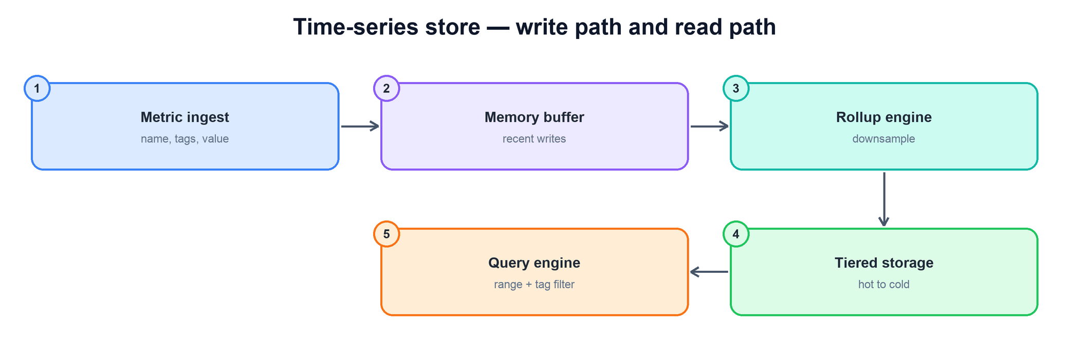
The stages:
- Metric ingest. Receivers accept batches of (name, tags, timestamp, value) points from agents running on every host. They resolve each point to its series id and route it onward. This layer is stateless and scales horizontally with the write load.
- Memory buffer. Recent points for each active series are held in an in-memory structure — the hot, write-optimized tier. Appending to an in-memory column is far cheaper than a disk write per point, and because reads of "the last few minutes" are the most common dashboard query, keeping recent data in memory serves them instantly. The buffer is backed by a write-ahead log so a crash does not lose unflushed points.
- Rollup engine. As the buffer fills or ages, its contents are downsampled and compressed before being flushed (covered next).
- Tiered storage. Flushed, compressed blocks land in durable storage organized from hot (recent, high-resolution, fast media) to cold (old, low-resolution, cheap media).
- Query engine. Reads fan out across the memory buffer and the storage tiers, stitching together recent and historical data to answer a query.
function write(point):
  series_id = index.resolve(point.name, point.tags)  # name + tags -> series
  wal.append(series_id, point.ts, point.value)       # durability first
  buffer[series_id].append(point.ts, point.value)    # hot in-memory append
  if buffer[series_id].full():
    rollup_and_flush(series_id)                       # downsample + compress
5. Rollups and Retention Tiers
Nobody needs per-second resolution for data that is two years old, and storing it that way would be wildly wasteful. The store therefore downsamples high-resolution data into progressively coarser resolutions as it ages, and pairs each resolution with a retention period. Recent data is kept fine-grained for a short time; old data is kept coarse but for a long time.
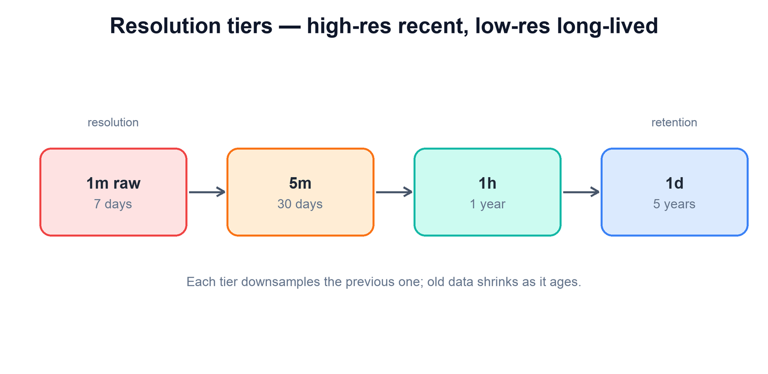
Downsampling reduces a window of fine points to one coarse point by applying an aggregate — typically average, min, max, and sum together, so a query can still ask for any of them. A 1-minute series rolled to 1-hour replaces sixty points with one. Because each tier is far smaller than the one below it, retaining a coarse tier for years costs a fraction of what retaining the raw tier for the same span would. The query layer transparently picks the finest tier that still covers the requested range and resolution, so a "last hour" query hits the raw tier while a "last year" query hits the daily tier.
| Resolution | Retention | Storage cost |
|---|---|---|
| 1 minute (raw) | ~7 days | Highest — but only for a short, recent window. |
| 5 minutes | ~30 days | One fifth of raw at the same span. |
| 1 hour | ~1 year | Cheap enough to keep a full year. |
| 1 day | ~5 years | Tiny — long-range history for almost nothing. |
6. Compression
Even with rollups, the raw tier holds an enormous number of points, so compression is what makes the whole thing economical. Time-series data compresses extraordinarily well because both its columns are highly regular, and the canonical techniques — popularized by the Gorilla in-memory store — exploit that regularity directly. The trick is to compress timestamps and values as two separate streams.
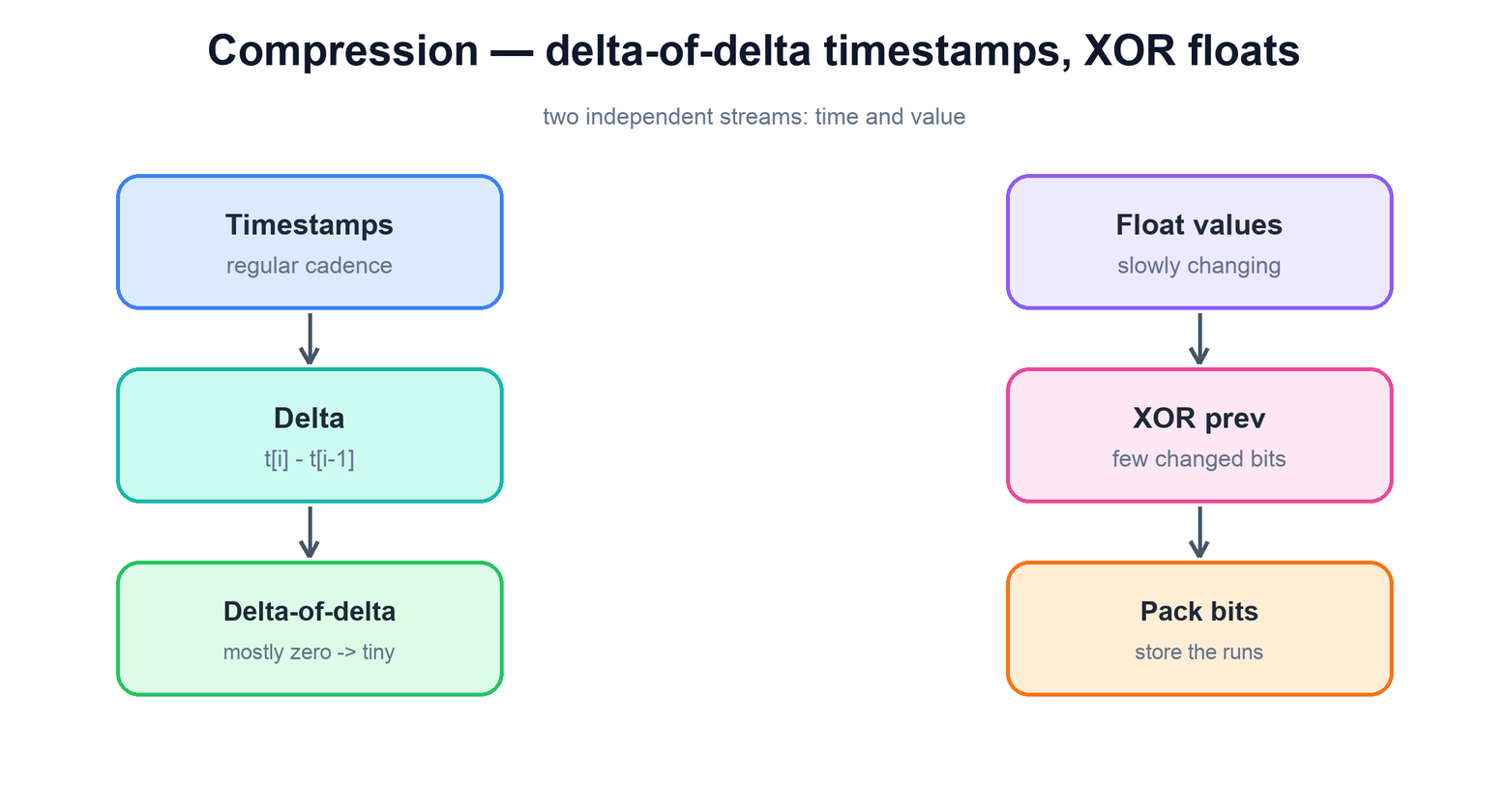
Delta-of-delta on timestamps. Points usually arrive at a fixed cadence — say every minute. The difference between consecutive timestamps (the delta) is therefore nearly constant, and the difference between consecutive deltas (the delta-of-delta) is almost always zero. Storing a long run of zeros takes almost no space, so a stream of regular timestamps collapses to a handful of bits per point instead of a full 64-bit timestamp.
XOR on values. Adjacent readings of a real metric tend to be close — CPU usage at 50.1% then 50.2%. XORing each float against the previous one yields a result that is mostly zero bits, with only a small middle band of differing bits. Storing just that band of meaningful bits, rather than the whole 64-bit float, shrinks slowly-changing series dramatically. When a value is unchanged, the XOR is all zeros and costs a single bit.
# timestamps: store the second difference (usually 0)
dod[i] = (ts[i] - ts[i-1]) - (ts[i-1] - ts[i-2])   # regular cadence -> 0

# values: XOR against previous, store only the changed bits
xor = bits(value[i]) ^ bits(value[i-1])            # mostly zero bits
store(leading_zeros(xor), meaningful_bits(xor)) # skip the zeros7. The Query Path
A query against a metrics store has a recognizable shape: it picks a metric, filters by tags, restricts to a time range, and aggregates. The engine answers it by turning that into a series selection plus a scan plus a fold.
- Series selection by tags. An inverted index maps each tag key-value pair to the set of series carrying it. A filter like
host=web42, status=200intersects the matching sets to find exactly the series to read. This is what makes "show me errors across all hosts in us-east" fast instead of a full scan. - Range scan. For each selected series, the engine reads the compressed (timestamp, value) blocks overlapping the requested time window, choosing the resolution tier that fits, and decompresses them.
- Aggregation. The points are folded — summed, averaged, rated for counters, or grouped across series — into the final result the dashboard plots. Grouping by a tag, for example summing request counts across all hosts per region, happens here.
function query(metric, tag_filter, start, end, agg):
  series = index.match(metric, tag_filter)     # inverted index intersection
  tier   = pick_resolution(start, end)         # finest tier covering the range
  result = []
  for s in series:
    points = storage.scan(s, tier, start, end) # decompress overlapping blocks
    result.append(aggregate(points, agg))      # avg / sum / rate / ...
  return combine(result, agg)                  # group across series
8. Read vs Write Separation
The write and read workloads have almost nothing in common, so a robust design keeps them on separate paths. Writes are a relentless, latency-sensitive append stream that must never stall; reads are spiky, often expensive range scans driven by humans opening dashboards and by alerting rules evaluating continuously. Letting a heavy read query contend with the ingest path is how a metrics system falls over exactly when an incident makes everyone open dashboards at once.
Separation shows up at several layers. The ingest tier and the query tier scale independently, so a surge of dashboard traffic does not slow ingestion and a write spike does not slow queries. The memory buffer serves recent reads directly without disturbing the flush pipeline. And because the data is immutable once flushed, historical reads can be served from the storage tiers with no coordination against ongoing writes at all — there are no locks to contend, since old blocks never change. The result is a system that keeps ingesting through a query storm and keeps serving queries through a write spike.
9. Summary
A metrics / time-series store is a specialist database whose every choice flows from a single observation: the data has a narrow, regular shape, and the workload is append-heavy writes with range-scan reads.
| Concern | Mechanism |
|---|---|
| What is a data point? | Metric name + tags + timestamp + value; name plus tags identifies one series. |
| How are values interpreted? | Gauges graphed directly; counters converted to a rate at read time. |
| What is the dominant scaling limit? | Cardinality — keep tags bounded, never label with unbounded ids. |
| How do we ingest at scale? | Append-optimized path: stateless ingest, in-memory buffer with a WAL, then flush. |
| How do we keep years of history cheaply? | Downsample into coarser resolutions with longer retention as data ages. |
| How do we make storage affordable? | Delta-of-delta timestamps and XOR float compression on regular series. |
| How do we answer a query fast? | Inverted tag index to select series, range scan the right tier, aggregate. |
| How do we stay stable under load? | Separate read and write paths; immutable flushed blocks need no read-write coordination. |