Designing a Search Autocomplete System
A system design interview guide to typeahead: how to return the most popular suggestions for a prefix in single-digit milliseconds, on every keystroke, by precomputing answers in a trie and rebuilding it offline from query logs.
Search autocomplete — also called typeahead or search-as-you-type — is the dropdown of suggested completions that appears the moment you start typing into a search box. It looks trivial from the outside, but it has a brutal performance profile: it fires on every keystroke, it must rank suggestions by popularity, and it has to feel instantaneous or it is useless. The trick that makes it work is to split the problem into two independent halves. An online query service answers "given this prefix, what are the top suggestions?" as fast as the network allows, and an offline data-gathering pipeline does all the heavy lifting — counting how often each query is searched and baking those counts into a data structure the query service can read in one hop. This guide walks through both halves, the trie that connects them, and how the whole thing scales.
Contents
1. Requirements and Scope
Before touching architecture, pin down exactly what the system must do. Autocomplete has a small functional surface but unusually demanding non-functional requirements, and the design is driven almost entirely by the latter.
| Requirement | What it means |
|---|---|
| Top-k suggestions | For a given prefix, return the k most relevant completions (typically 5 to 10). Not all completions — just the best few that fit in the dropdown. |
| Ranked by popularity | Suggestions are ordered by how often people actually search them (their historical frequency), so the most likely intent floats to the top. |
| Extremely fast | The query fires on every keystroke, so a single request must return in a few milliseconds. A common target is a latency budget around 100 ms end to end, including the network round trip. |
| Prefix match | Suggestions must start with what the user has typed so far. (Fuzzy or mid-word matching is a separate, harder feature usually left out of scope.) |
| Fresh enough | Rankings should reflect real search trends, but they do not need to be real-time. Trends shift over days and weeks, not seconds. |
It is worth being explicit about the load. If a user types a ten-character query, that is up to ten autocomplete requests for a single search. Multiply by every user typing into the box and the read volume dwarfs almost any other endpoint in the product. The flip side is that writes are rare and can be deferred — nobody is editing the suggestion set interactively. That asymmetry (massive reads, lazy writes) is the single most important fact about the design, and it is what licenses the offline-pipeline approach.
2. Two Subsystems
The cleanest way to reason about autocomplete is to separate the read path from the build path completely. They have opposite characteristics — one is latency-critical and runs constantly, the other is throughput-oriented and runs occasionally — so they get different designs, different hardware, and different scaling stories.
- The query service (online). A request comes in carrying a prefix; the service looks up the precomputed top-k for that prefix and returns it. This path does almost no computation at request time — that is the whole point. All the expensive ranking work has already been done.
- The data-gathering pipeline (offline). This consumes the raw stream of what people searched, aggregates it into per-query frequency counts, builds the data structure the query service reads (a trie), and periodically publishes a fresh copy. It is allowed to be slow because it runs out of the request path.
The contract between the two halves is just the data structure: the pipeline produces it, the query service consumes it. Because the query service only ever reads a finished, immutable snapshot, it never blocks on a build and never sees a half-updated structure. Keeping these subsystems decoupled is what makes the read path simple enough to be fast.
3. The Trie and Cached Top-k
The data structure at the heart of autocomplete is the trie (pronounced "try"), also called a prefix tree. A trie stores strings character by character: the root is the empty prefix, each edge is a character, and the path from the root to any node spells out a prefix. The word best shares its b, be, and bes nodes with bee and beer, so common prefixes are stored exactly once. Every node corresponds to a prefix, and the subtree beneath a node contains every complete query that starts with that prefix.
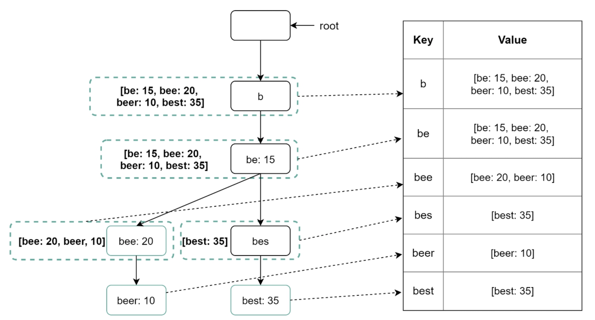
The naive way to answer a query is to walk down the trie to the node for the prefix, then traverse its entire subtree to collect every completion, sort them by frequency, and return the top k. That works, but it is far too slow. A short prefix like b can have an enormous subtree — potentially every query in the corpus that starts with b — and traversing and sorting it on every keystroke is exactly what the latency budget forbids.
The key optimization is to precompute and cache the top-k suggestions at each node. When the trie is built offline, each node stores, alongside its children, a small fixed-size list of the best k completions in its subtree, already sorted by popularity. With that in place, a query collapses to: walk to the prefix node, read its cached list, return it. The traversal-and-sort is gone entirely — answering a query is a single node lookup followed by reading a list of k strings.
function query(prefix):                   # online, hot path
  node = root
  for ch in prefix:
    node = node.children[ch]
    if node is None:
      return []                           # no such prefix
  return node.top_k                        # precomputed, already sorted
This is a deliberate space-for-speed tradeoff. Storing a top-k list at every node duplicates data heavily: the completion best may appear in the cached list of b, be, bes, and best. The trie therefore consumes considerably more memory than one that only stored the words themselves. In return, query time drops from "proportional to the size of the subtree" to "proportional to the length of the prefix" — and prefixes are short and bounded, so in practice it is effectively constant. For a system whose entire reason to exist is read latency, paying memory to buy speed is the right call. If memory becomes a real constraint, a common compromise is to cache top-k only at nodes above some prefix length and fall back to a bounded traversal for the long, rare prefixes.
| Approach | Query cost | Memory |
|---|---|---|
| Trie + subtree traversal | Walk to node, then traverse and sort the whole subtree. Slow for short prefixes. | Minimal — stores each query once. |
| Trie + cached top-k per node | Walk to node, read the cached list. Effectively constant. | Higher — each completion is duplicated across all of its ancestor prefixes. |
4. The Data-Gathering Pipeline
The trie does not appear from nowhere; it is the output of an offline pipeline that turns raw search activity into ranked suggestions. The pipeline runs on its own schedule, well away from the query service, and publishes finished snapshots for the query service to pick up.
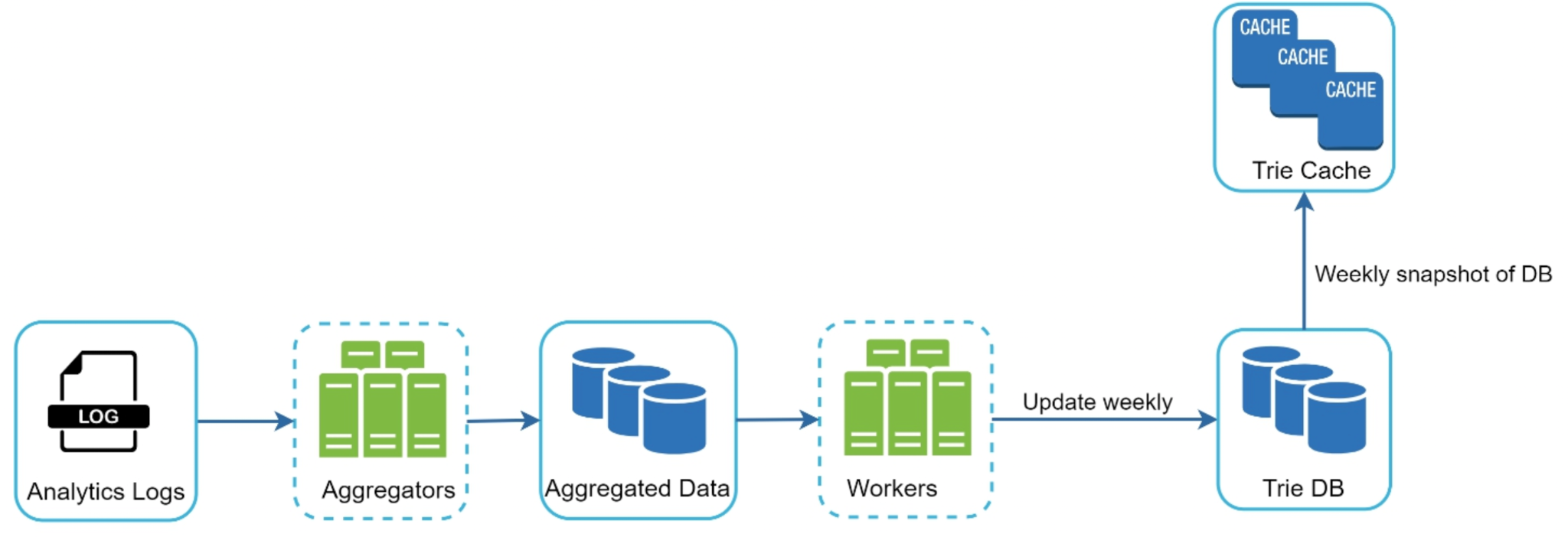
The stages are:
- Analytics logs. Every search the product serves is logged as a raw event — the query string, and usually a timestamp. This is an append-only firehose; it is the ground truth for what is actually popular.
- Aggregators. Jobs read the raw logs and collapse them into frequency counts: how many times each distinct query string was searched over the chosen window. This is a classic group-by-and-count, run as a batch (or windowed) job because the log volume is huge.
- Aggregated data. The result is a compact table of
(query, frequency)pairs — far smaller than the raw logs, since millions of events collapse into one row per distinct query. - Workers. A set of build workers read the aggregated table and construct the trie. As they insert each
(query, frequency)pair they also update the cached top-k lists on the path of nodes leading to that query, so the finished trie has its per-node suggestion lists already populated. - Trie DB. The built trie is persisted to durable storage — the source of truth for the current suggestion data. Holding it in a database (rather than only in memory) means a build can be reproduced, inspected, and reloaded after a restart.
- Trie cache (snapshot). Periodically — say weekly — a snapshot of the trie is loaded into the in-memory cache that the query service actually reads from. Publishing a fresh snapshot is how new rankings go live.
# offline build, runs on a schedule (e.g. weekly)
function build_trie(aggregated):           # (query, frequency) rows
  root = new_node()
  for (query, freq) in aggregated:
    node = root
    for ch in query:
      node = node.children.setdefault(ch, new_node())
      offer_to_top_k(node, query, freq)    # keep best k on the path
  persist(root, trie_db)                    # durable source of truth
  publish_snapshot(trie_db, trie_cache)     # swap in for the query service
The defining choice here is that the rebuild is offline and periodic rather than near-real-time, and for autocomplete that is exactly right. Popular-query rankings change slowly: the set of things people search for, and their relative order, drifts over days and weeks, not seconds. A suggestion that was popular yesterday is almost certainly still popular today, so serving rankings that are a few days stale costs essentially nothing in quality. A real-time pipeline that updates the trie on every search would add enormous complexity — concurrent updates to cached top-k lists, contention with the read path, far more infrastructure — to chase freshness the product does not need. Rebuilding periodically lets the build be a clean, batch-shaped, restartable job, and lets the query service treat each published snapshot as an immutable thing it never has to mutate.
5. Serving and Scale
The query service exists to do one thing quickly: take a prefix and return its cached top-k. Everything about how it is deployed serves that goal.
Cache the trie in memory. The whole point of the precomputed top-k is defeated if reading a node requires a disk seek. The serving copy of the trie lives entirely in RAM, so a query is a handful of in-memory pointer hops plus reading a short list. The Trie DB is the durable backing store; the Trie cache is the fast serving copy, and the query service reads only the latter.
Shard when the trie outgrows one machine. A trie with cached top-k at every node can grow too large for a single server's memory. The natural way to split it is by prefix — for example, route prefixes starting with a–m to one shard and n–z to another, or shard on the first one or two characters. Because a prefix uniquely determines which shard owns it, the query router can send each request directly to the right shard with no fan-out. The risk is skew: some first letters are far more common than others, so shards are sized by estimated load rather than splitting the alphabet evenly.
Replicate for read throughput. Sharding handles a trie that is too big; replication handles a read volume that is too high. Since the serving trie is read-only between snapshot swaps, replicas are trivial to create — every replica of a shard holds an identical copy, and reads are load-balanced across them. There is no write-consistency problem to worry about because nothing writes to a replica during serving; updates arrive only as a whole new snapshot, which can be rolled out replica by replica.
| Technique | Problem it solves | Why it is cheap here |
|---|---|---|
| In-memory trie | Per-query latency | Query is pointer hops + a short list read; no disk in the hot path. |
| Shard by prefix | Trie too large for one machine | Prefix determines the shard, so routing is direct with no fan-out. |
| Replicate shards | Read volume too high | Read-only snapshots replicate freely; no write-consistency to manage. |
6. Client-Side Concerns
A surprising amount of autocomplete's perceived speed and its load profile are controlled in the browser, before a request ever reaches the server. The client is the first line of defense for the latency budget.
- Debounce keystrokes. Firing a request on every single keypress is wasteful — a fast typer generates a burst of prefixes most of which are obsolete before a response returns. Debouncing waits for a short pause in typing (say 50–100 ms) before sending a request, so only meaningful prefixes hit the server. This cuts request volume dramatically and avoids showing flickering, out-of-order results.
- Cache recent results in the browser. Suggestions for a prefix rarely change between keystrokes, so the client can cache responses locally. When the user deletes a character and retypes, or when one prefix is a continuation of a cached one, the dropdown can be served instantly from the browser with no network call at all.
- Respect a tight latency budget. The dropdown has to feel like it is keeping up with the user. With a budget on the order of 100 ms for the full round trip, every layer has to be lean: a debounce window short enough not to feel laggy, an in-memory server lookup, and a small response payload (just
kstrings). Responses can also carry cache headers so the browser and any CDN edge can reuse them, shaving the round trip on repeated prefixes.
7. Summary
Autocomplete is a study in pushing work out of the request path. Almost every design decision trades build-time or memory cost for read-time speed, because the read path is the only thing the user feels.
| Concern | Mechanism |
|---|---|
| How is a query answered fast? | Walk the trie to the prefix node and return its precomputed top-k list — a single node lookup, no subtree traversal. |
| What is the core data structure? | A trie (prefix tree) where each node caches the top-k most popular completions in its subtree, pre-sorted by frequency. |
| What is the cost of that cache? | Extra memory: each completion is duplicated across all of its ancestor prefix nodes. Space traded for speed. |
| Where do rankings come from? | An offline pipeline: analytics logs → aggregators → aggregated frequencies → build workers → Trie DB. |
| How do new rankings go live? | A periodic (e.g. weekly) snapshot of the trie is published into the in-memory Trie cache the query service reads. |
| Why periodic, not real-time? | Popular-query trends drift over days, not seconds, so stale-by-days rankings are fine and avoid huge complexity. |
| How does it scale? | Trie cached in memory; sharded by prefix when too large; replicated for read throughput since snapshots are read-only. |
| What does the client do? | Debounce keystrokes, cache recent results, discard stale responses, and stay inside a tight latency budget. |