Designing a Proximity Service
A system design interview guide to building a Yelp-style "nearby places" service that, given a location, returns the businesses around you fast — by indexing the world spatially instead of scanning every row.
A proximity service answers a deceptively simple question: "what is near me?" Type that into a maps or reviews app and you expect a list of restaurants, gas stations, or pharmacies within a few kilometers, sorted by distance, in well under a second. The naive way to compute this — store every place with its latitude and longitude and, on each request, look at all of them — falls over the moment you have millions of places and thousands of queries per second. The interesting part of the design is not the distance formula; it is the spatial index that lets you look at a few hundred candidate places instead of all of them. This guide builds up from why the obvious query does not scale, through the indexing options an interviewer expects you to compare, to the read-heavy serving architecture that ties it together.
Contents
1. The Range Query Problem
Start with the design everyone reaches for first: a table of places, each with a latitude and a longitude, and a query that asks for everything inside a bounding box around the user. In SQL it looks like a simple range filter on two columns.
SELECT id, name, lat, lng FROM places
WHERE lat  BETWEEN :user_lat - d AND :user_lat + d
  AND lng  BETWEEN :user_lng - d AND :user_lng + d;
This works on a small dataset and is completely correct. The trouble is performance at scale. Latitude and longitude are two independent dimensions, and a standard B-tree index can only order rows along one of them at a time. An index on lat narrows the search to a horizontal band of the planet; an index on lng narrows it to a vertical band. Neither narrows it to the small square you actually want. The database ends up scanning one long band and checking the other coordinate row by row, so the work grows with the total number of places, not with how many are genuinely nearby.
The root cause is that nearness in two dimensions has no natural single ordering. Two places can be close on the map yet far apart in any one-column sort. To make "near me" cheap, you need a way to map 2D location into something a single index can order, so that points which are close on the ground end up close in the index. That is exactly what spatial indexes do, and the three approaches below are the ones an interviewer will want you to weigh against each other.
2. Geohash
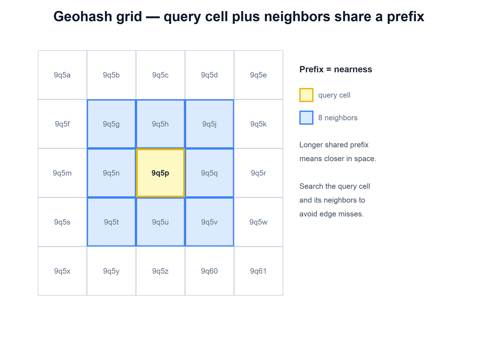
A geohash encodes a latitude/longitude pair into a short string of letters and digits. It works by repeatedly cutting the world in half — first by longitude, then latitude, then longitude again — and recording, with one bit each time, which half the point falls in. Those bits are then grouped and base-32 encoded into a string. The crucial property is that a shared prefix means spatial nearness: two places whose geohashes start with the same characters sit inside the same region of the map, and the longer the shared prefix, the smaller that region and the closer they are.
This turns the 2D problem into a 1D one. Each place gets a geohash string, you store it as an indexed column, and "find places near a point" becomes "find places whose geohash shares the query's prefix." Because the strings sort lexicographically, neighbors in space are mostly neighbors in the sorted index, so a prefix scan returns a tight set of candidates.
The length of the geohash controls precision. A short prefix covers a large area (good for a coarse "what city is this" lookup); a longer prefix pins down a block-sized cell. You choose the precision to match the search radius — long enough that a cell is roughly the size of the area you care about.
| Geohash length | Approx. cell size | Use |
|---|---|---|
| 4 characters | ~20 km | City-level grouping |
| 5 characters | ~5 km | Neighborhood search |
| 6 characters | ~1 km | "Near me" walking radius |
| 7 characters | ~150 m | Block-level precision |
One sharp edge worth mentioning in an interview: two points can be physically adjacent yet fall on opposite sides of a major cut, so their geohashes share little or no prefix (the classic case is points straddling the equator or a longitude boundary). That is why a correct search never relies on the query cell alone — it always also examines the neighboring cells, which is the standard fix for this boundary problem.
# index a place by its geohash prefix
function index_place(place):
  place.geohash = geohash_encode(place.lat, place.lng, precision=6)
  db.places.insert(place)            # geohash column is indexed

# candidate lookup = prefix match on the query cell
function candidates(lat, lng):
  cell = geohash_encode(lat, lng, precision=6)
  return db.places.where("geohash LIKE :p", p = cell + "%")
3. Quadtree
A quadtree takes a different tack. Instead of fixed-size cells, it recursively subdivides space only where it is crowded. Start with one square covering the whole map. Whenever a square holds more than some threshold of places, split it into four equal quadrants and push the places down into them; repeat for any quadrant that is still too full. Empty oceans stay as one big node, while a dense downtown ends up subdivided many levels deep.
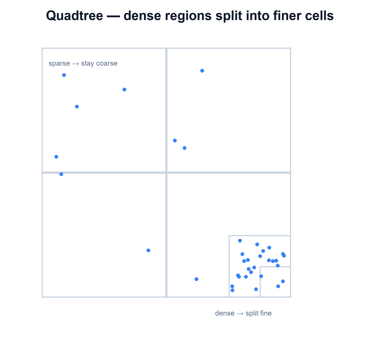
The payoff is adaptivity. Every leaf node holds roughly the same small number of places regardless of how dense the real world is there, so a query that descends to a leaf always gathers a bounded, predictable candidate set. A fixed grid cannot do this: pick cells small enough for downtown and rural cells are nearly empty; pick cells large enough for the countryside and a city cell holds tens of thousands of places. The quadtree sidesteps that trade-off by varying resolution with density.
The cost is that a quadtree is a tree you typically hold in memory and must build and rebalance as data changes, whereas geohashes are just strings you can store in any ordinary indexed column. In an interview, the clean contrast is: geohash trades adaptivity for simplicity; the quadtree trades simplicity for adaptivity.
function search(node, query_box):
  if not node.bounds.intersects(query_box):
    return []
  if node.is_leaf():
    return [p for p in node.places if query_box.contains(p)]
  results = []
  for child in node.children:        # NW, NE, SW, SE
    results += search(child, query_box)
  return results
4. Grid and Cell Systems
The third family treats the planet as a set of named cells produced by a well-defined cell system, the best known being Google's S2. S2 projects the sphere onto the six faces of a cube and recursively subdivides each face into a hierarchy of cells, giving every cell a 64-bit id. Like a geohash, an S2 cell id is a single sortable number whose ordering preserves locality, so nearby cells have nearby ids; like a quadtree, the cells form a hierarchy you can query at coarse or fine levels.
What a mature cell system buys you over a hand-rolled grid is correctness on a sphere and a clean, ready-made notion of "the cells covering this region." Given a query area, the library returns the small set of cell ids that cover it, and you look up places tagged with those ids. The two-column lat/long range query becomes a set-membership test on a handful of cell ids — exactly the kind of thing a single index handles well.
| Approach | Cell sizing | Storage | Best when |
|---|---|---|---|
| Geohash | Fixed, by prefix length | Plain indexed string column | Simple, uniform-ish data; easy to store in any DB |
| Quadtree | Adaptive to density | In-memory tree | Very uneven density; bounded candidate sets matter |
| Grid / S2 | Hierarchical, sphere-correct | Indexed cell-id column | Large scale, want a battle-tested covering library |
5. The Search Algorithm
Whichever index you pick, the runtime search follows the same shape, and being able to recite it cleanly is half the interview. The key idea is that the spatial index does the coarse filtering — narrowing the world to a small candidate set — and a cheap exact computation does the fine filtering afterward. The index gets you close; the distance formula makes it precise.
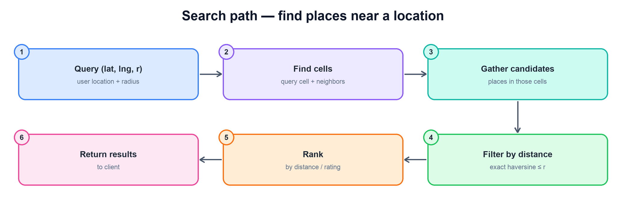
Step by step:
- Compute the query cell. Encode the user's location at the precision matching the search radius — a geohash prefix, a quadtree leaf, or an S2 covering.
- Add the neighbors. Include the adjacent cells so you do not miss places sitting just across a boundary. This is the standard fix for the edge problem all cell schemes share.
- Gather candidates. Pull every place tagged with one of those cells. This is a small set — bounded by cell size or quadtree leaf capacity — not the whole table.
- Filter by exact distance. For each candidate, compute the true great-circle (haversine) distance to the user and discard anything beyond the radius. The cells are square-ish; the radius is a circle, so this trims the corners.
- Rank and return. Sort the survivors by distance (and possibly rating or relevance) and return the top results.
function nearby(lat, lng, radius):
  cells      = cells_for(lat, lng, radius)        # query cell + neighbors
  candidates = []
  for cell in cells:
    candidates += index.places_in(cell)           # coarse: small set
  results = []
  for p in candidates:
    d = haversine(lat, lng, p.lat, p.lng)         # fine: exact distance
    if d <= radius:
      results.append((d, p))
  results.sort()                                   # nearest first
  return [p for _, p in results]
6. Handling Uneven Density
Real-world places are not spread evenly. A dense city center may hold orders of magnitude more businesses per square kilometer than a rural area, and this lopsidedness is what punishes a one-size-fits-all index. With fixed cells, a downtown cell can return tens of thousands of candidates while a rural cell returns three — the same query costs wildly different amounts depending on where you stand.
This is precisely where the quadtree earns its keep: because it splits busy regions finely and leaves empty regions coarse, every leaf holds roughly the same bounded number of places. A query in a dense downtown descends a few extra levels and still lands on a small candidate set, so cost stays predictable everywhere. The fixed-grid alternative forces an awkward compromise on cell size, and the usual mitigations — capping results per cell, or maintaining different precisions for different regions — are really just approximations of what the quadtree does for free.
| Region | Fixed grid cell | Quadtree behavior |
|---|---|---|
| Dense downtown | One cell, thousands of candidates | Splits deep; each leaf stays small |
| Suburb | One cell, a few hundred | Splits a couple of levels |
| Rural / water | One cell, near-empty | Stays a single coarse node |
7. Precomputation and Caching
A proximity service is overwhelmingly read-heavy, and most of the work is the same from request to request: the set of places near a given area changes slowly, while queries for that area arrive constantly. That mismatch is an invitation to precompute and cache. Rather than recomputing candidate sets on every request, you can keep per-cell results warm and serve repeated queries straight from memory.
- Index at write time. Compute each place's cell id (geohash, quadtree leaf, or S2 id) when the place is created or moved, not at query time. The expensive encoding happens once per place, not once per request.
- Cache by cell. Use the cell id as a natural cache key. The list of places in a popular cell is a perfect candidate for an in-memory cache, since many users querying the same neighborhood hit the same cells.
- Tolerate slight staleness. Businesses do not open and close by the second, so a cache that lags by minutes is fine. This loose freshness requirement is what makes aggressive caching safe.
8. Serving Architecture
Putting it together, the production shape reflects the read-heavy nature of the workload: a tier of stateless servers, a cache in front of the spatial index, and a separate, lower-traffic path for updating places. Reads scale horizontally; writes are comparatively rare and can be handled more deliberately.
- Stateless query servers. They receive "nearby" requests, compute the query cells, consult the cache, fall back to the spatial index in the database on a miss, run the exact-distance filter, and return ranked results. Being stateless, they scale out simply behind a load balancer.
- Spatial index + cache. The geohash/quadtree/S2 index lives in the database (or in memory for a quadtree), fronted by a cache keyed on cell id so hot neighborhoods are served without touching the database.
- Place data store. The source of truth for place details — name, category, rating, hours — alongside the cell id used for lookups.
- Write/ingestion path. A separate path adds and updates places, recomputing the cell id and invalidating any cached cells. Kept distinct from reads so a burst of edits never slows queries.
The recurring theme is the split between a cheap, cacheable coarse lookup and an exact fine filter, served by a fleet that is mostly read replicas and caches. That separation — plus indexing at write time so reads stay light — is what lets a proximity service answer "what is near me?" in milliseconds across millions of places.
9. Summary
A proximity service is fundamentally a spatial-indexing problem dressed up as a search feature. The design is a chain of choices that each reduce work:
| Concern | Mechanism |
|---|---|
| Why doesn't a lat/long range query scale? | Two independent columns; a 1D index can't narrow both, so cost grows with total places. |
| How do we make nearness one-dimensional? | Geohash: encode location into a string whose shared prefix means spatial nearness. |
| How do we cope with uneven density? | Quadtree: recursively subdivide only the crowded regions so every leaf stays small. |
| What if we want a sphere-correct, hierarchical scheme? | A cell system like S2: 64-bit cell ids that preserve locality and cover any region. |
| How does a search actually run? | Compute query cell + neighbors, gather candidates, filter by exact distance, rank. |
| Why include neighboring cells? | Places near a cell boundary would otherwise be missed; neighbors fix the edge problem. |
| How do we keep latency low under load? | Index at write time, cache results per cell, tolerate slight staleness. |
| What does the serving tier look like? | Stateless query servers + cache over the index, with a separate write path. |