OpenObserve — Internal Architecture
A developer's guide to how OpenObserve actually works under the hood: the node roles, the schema-on-ingest pipeline, columnar Parquet on object storage, and how a query prunes its way down to the few files it actually needs.
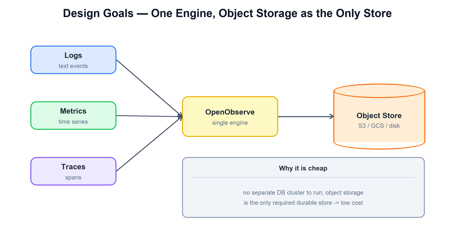
OpenObserve is an observability platform — logs, metrics, and traces in one engine. Its design is built around a single, simple bet: object storage is the only durable store you need. There is no separate time-series database cluster, no dedicated search cluster, and no per-node attached disk that holds the source of truth. Data lands as compressed columnar Parquet files on an object store (S3, GCS, Azure Blob, MinIO, or even a local filesystem), and every other component is effectively a stateless worker that reads and writes those files. That choice — borrowing the data-lake storage model and pairing it with an Apache Arrow / DataFusion query engine — is what makes it cheap to run and is the thread that ties the rest of the architecture together.
Contents
1. Design Goals and Core Ideas
Every internal decision in OpenObserve traces back to a small set of goals. Keeping them in mind makes the rest of the architecture predictable.
| Goal | How OpenObserve achieves it |
|---|---|
| Cheap observability | Object storage is the only required durable store. No separate database cluster, no expensive local SSDs holding the source of truth. Data is compressed columnar Parquet, so storage and scan costs stay low. |
| Unified signals | Logs, metrics, and traces all flow through one ingestion pipeline and land in the same Parquet-on-object-store format, queried by one engine. There is no separate stack per signal type. |
| Stateless compute | Node roles (router, ingester, querier, compactor) keep no durable state of their own. Everything that must survive a restart lives in the object store or the metadata store, so compute scales independently. |
| Schema-on-ingest | You do not declare a schema up front. Columns are inferred from the first records and extended as new fields appear, so any JSON shape can be ingested immediately. |
| SQL-first querying | Queries are SQL (and PromQL for metrics), planned and executed by DataFusion over Arrow. The same engine serves logs, metrics, and traces. |
2. Architecture
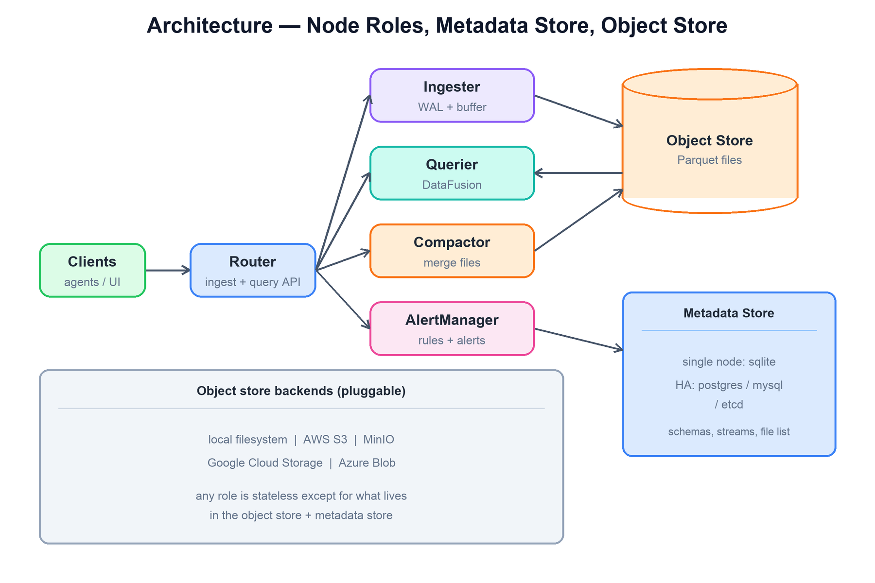
OpenObserve runs in two deployment shapes from the same binary. In single-node mode every role runs in one process backed by an embedded SQLite metadata store and a local-disk object store. In HA (cluster) mode the roles run as separate, independently scalable deployments, the metadata store moves to PostgreSQL, MySQL, or etcd, and the object store is a real bucket (S3, GCS, Azure, or MinIO).
The components are:
- Router: the front door. It terminates the ingest and query HTTP APIs, handles authentication, and forwards each request to the appropriate role — ingest traffic to ingesters, query traffic to queriers. It holds no data.
- Ingester: receives incoming records, writes them to a write-ahead log for durability, accumulates them in an in-memory buffer, and periodically flushes that buffer to a Parquet file on the object store. It also performs schema inference.
- Querier: executes queries. It asks the metadata store which Parquet files are relevant, fetches only those (and only the needed columns) from the object store, and runs the plan with DataFusion over Arrow.
- Compactor: a background role that merges many small Parquet files into fewer larger ones, applies downsampling for metrics, and enforces retention by deleting expired files.
- AlertManager: evaluates alert rules on a schedule (running them as queries) and dispatches notifications when conditions fire.
Two stores sit behind the roles:
- Metadata store: the small, consistent catalog. It holds organizations, stream definitions, inferred schemas, the list of Parquet files and their statistics, alert rules, and cluster membership. Single-node uses embedded SQLite; HA uses PostgreSQL / MySQL / etcd. This is the only component that needs a real database, and it stays tiny because it stores pointers and metadata, never the observability data itself.
- Object store: the bulk durable store for all Parquet files. Pluggable backend: local filesystem, AWS S3, MinIO, Google Cloud Storage, or Azure Blob. Everything large lives here.
3. Data Model
The data model has three levels. An organization is the top-level tenant boundary — it isolates data, users, and quotas. Inside an organization you have streams, which are the equivalent of tables. Each stream has a type: logs, metrics, or traces. A stream is a sequence of records sharing a schema and a retention policy.
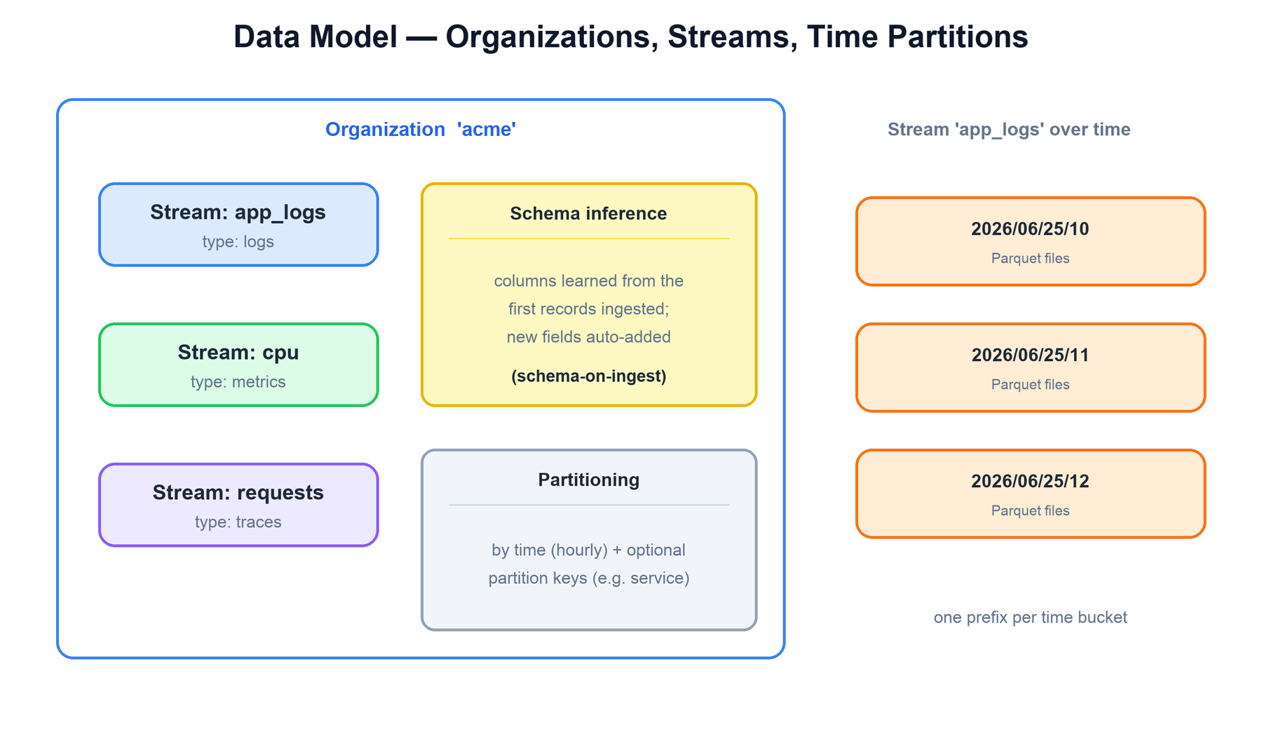
Schema inference is what makes ingestion frictionless. You do not run a CREATE TABLE. The first records to arrive on a stream define its columns and their types; when a later record carries a field the schema has not seen, the column is added and old rows simply have a null for it. This is schema-on-ingest — the schema is a living description maintained in the metadata store, not a fixed contract.
Partitioning is what makes querying fast. Every stream is partitioned by time (records are grouped into time buckets, typically hourly) and optionally by one or more partition keys (for example, a service or k8s_namespace column). Partitioning is expressed in the object-store key layout — each partition is its own prefix:
# object key layout for a partitioned stream
org/acme/logs/app_logs/
  2026/06/25/10/service=api/  # time bucket + partition key
    7f3a...parquet
    9b21...parquet
  2026/06/25/10/service=web/
    a44c...parquet
  2026/06/25/11/service=api/
    ...
Because partitions are encoded in the key prefix, a query with a time range and a service filter can be narrowed to a handful of prefixes before any file is opened. That is the first and cheapest layer of pruning.
4. Storage Format
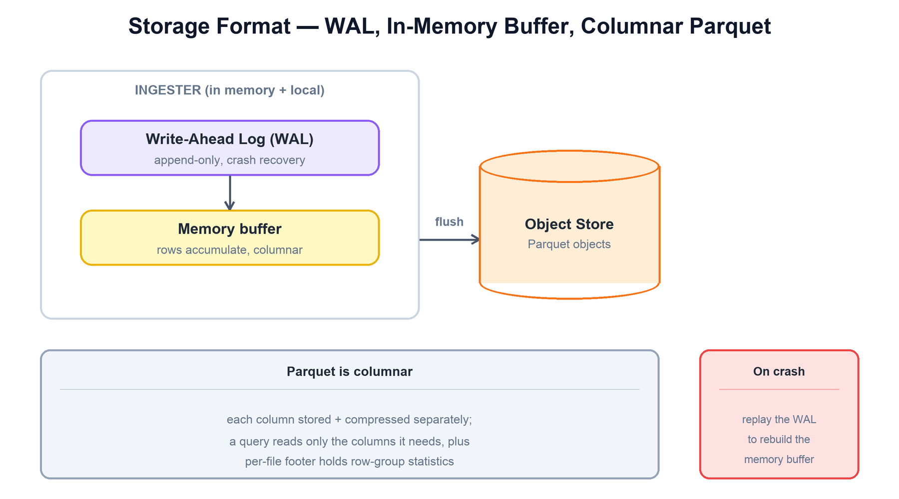
On the object store, all data is Apache Parquet — a columnar file format. Inside a Parquet file the values of each column are stored together and compressed independently, and the file is divided into row groups, each carrying per-column statistics (min, max, null count) in its footer. Columnar layout is the right fit for observability queries, which usually touch a few columns out of hundreds and filter on a small number of them.
The write side of the storage engine has three structures, the same shape as a log-structured store:
- Write-ahead log (WAL): an append-only file on the ingester's local disk. Its only job is durability. A record is acknowledged once it is in the WAL, so an ingester crash before the next flush loses nothing — the WAL is replayed on restart to rebuild the buffer.
- In-memory buffer (memtable): incoming records accumulate here, organized for columnar conversion. This is where schema inference happens and where data lives between flushes.
- Parquet file: when the buffer hits a size or time threshold, it is converted to a compressed columnar Parquet object and written to the object store. Like an SSTable, a Parquet file is immutable once written — it is never modified in place, only superseded and eventually compacted away.
The footer of every Parquet file is itself an index. Alongside the row-group statistics, OpenObserve records each file's overall min/max for the timestamp and partition columns in the metadata store, so the planner can reason about a file without reading it.
5. Ingestion Path
Ingestion is a straight pipeline. A record is durable the moment it is in the WAL; everything after that — buffering, Parquet conversion, the object-store upload — happens asynchronously and does not block the acknowledgement.
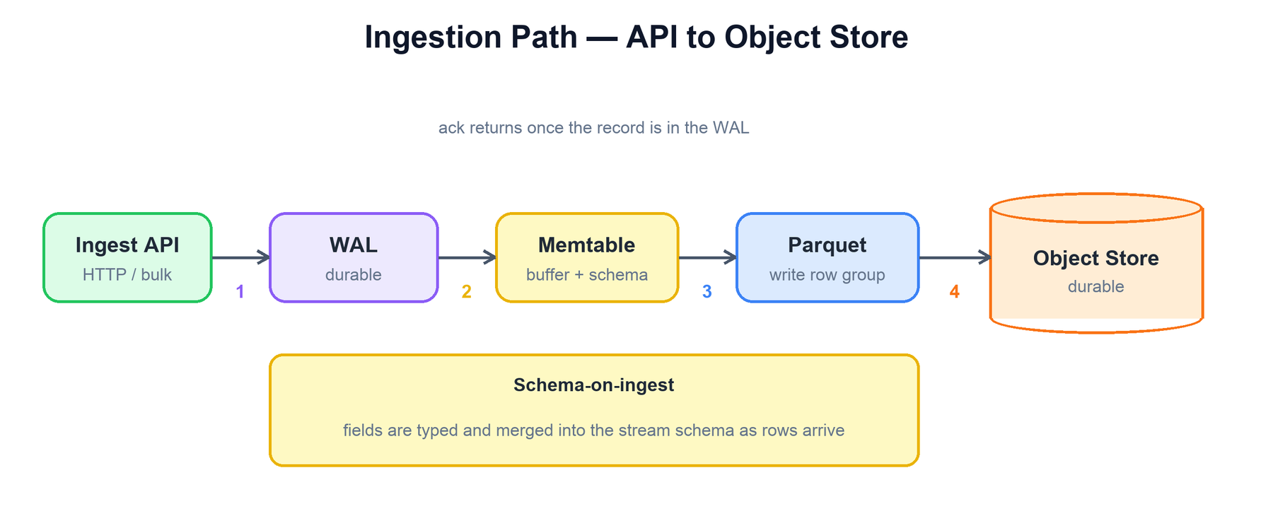
The sequence inside an ingester is:
function ingest(stream, records):
  for r in records:
    schema = infer_and_merge(stream, r)   # 1. schema-on-ingest
    wal.append(stream, r)                  # 2. durable; ack can return now
    buffer[stream].add(r)                  # 3. in-memory, columnar
  ack()                                    # client released after WAL write

  # asynchronously, on size/time threshold:
  if buffer[stream].should_flush():
    file = buffer[stream].to_parquet()     # 4. compress, columnar
    key  = partition_key(stream, file)     # time + partition keys
    object_store.put(key, file)            # upload to S3/GCS/...
    metadata.register_file(key, file.stats)  # min/max, rows, columns
    wal.truncate(covered_by(file))
The key detail is the order: durability (WAL) comes before visibility (buffer) and long before the Parquet flush. The flush registers the new file and its statistics in the metadata store in the same step, which is what makes the file immediately discoverable by queriers and prunable by the planner.
6. Indexing & Pruning
OpenObserve does not scan everything. The whole performance story is about reading as few bytes from the object store as possible, because object-store reads are the slow and metered part of a query. It does this with layered pruning, from coarse to fine.
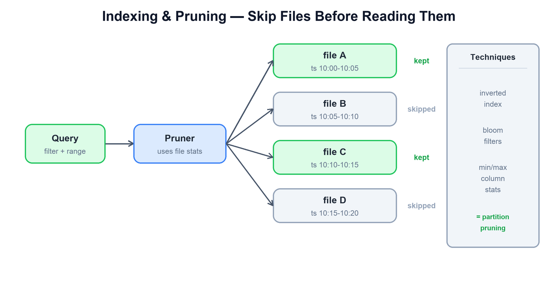
The layers, applied in order:
| Layer | Granularity | What it eliminates |
|---|---|---|
| Partition pruning | prefix / file | Time-range and partition-key filters narrow the candidate set to a few object-store prefixes before any file is touched. |
| Min/max column stats | file & row group | Each Parquet file (and each row group) carries per-column min/max. If a filter's value falls outside a file's range, the whole file is skipped. |
| Bloom filters | file | For high-cardinality equality filters (e.g. a specific trace_id), a bloom filter says "this value is definitely not here" so the file is skipped without reading it. |
| Inverted index | terms within a file | For full-text search over log fields, an inverted index maps terms to the records that contain them, so a text query reads only matching rows rather than scanning the column. |
Critically, the first three layers run on metadata only — the planner consults statistics held in the metadata store and the Parquet footers, deciding which files matter before downloading a single byte of column data. A query against a stream holding thousands of files commonly reads only a handful.
7. Query Path
A query is SQL (or PromQL for metrics). It is parsed into a logical plan, pruned down to a file set, then executed in parallel by queriers that fetch only the needed Parquet from the object store and run the plan with DataFusion over Arrow record batches.
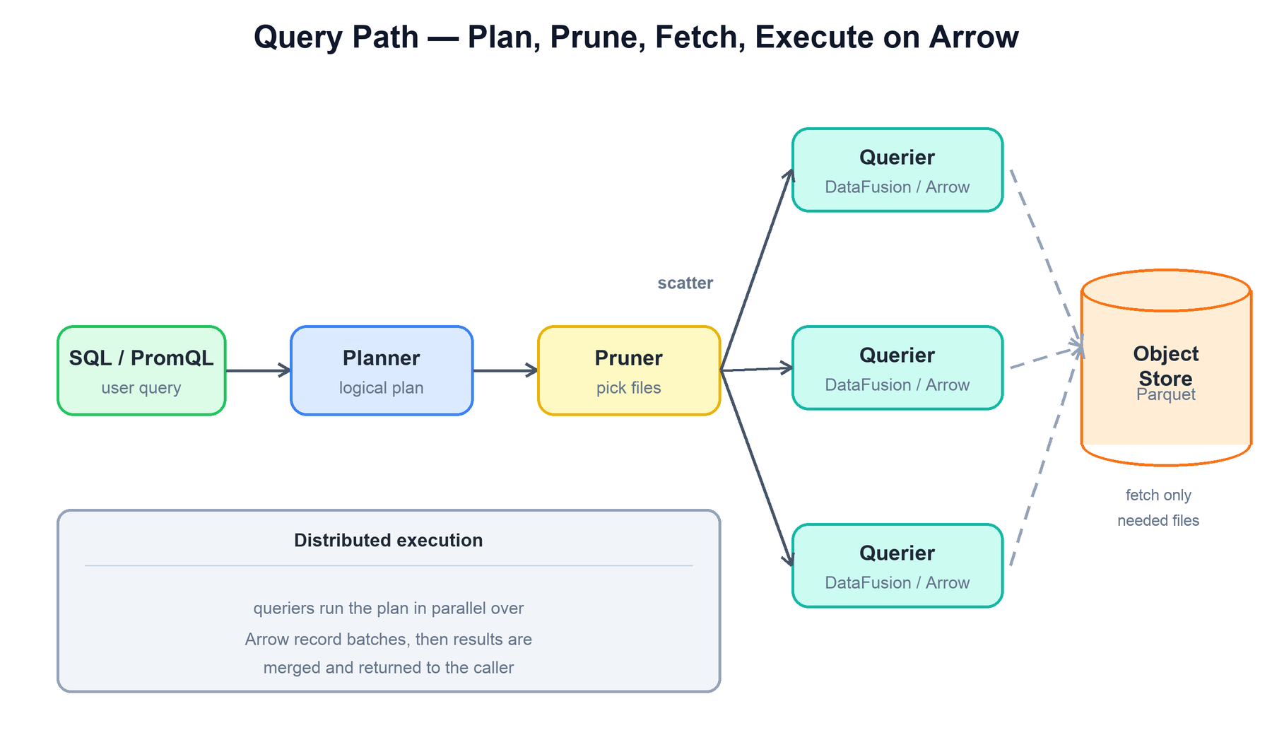
The end-to-end flow is:
function query(sql):
  plan  = planner.build(sql)              # logical plan + filters
  files = prune(plan, metadata)           # partitions + min/max + bloom
  shards = split(files, num_queriers)     # scatter the file set
  partials = []
  for q in queriers:                      # run in parallel
    partials += q.execute(plan, shards[q])
  return merge(plan, partials)            # gather + final aggregation

# inside a single querier:
function execute(plan, files):
  for f in files:
    cols  = f.read_columns(plan.projected_columns)  # only needed columns
    batch = arrow.decode(cols)            # Parquet -> Arrow
    emit(datafusion.run(plan, batch))     # filter / aggregate
Two things keep this fast. First, scatter-gather: in HA mode the pruned file set is split across many queriers, so a large scan parallelizes across machines and the partial results are merged at the end. Second, columnar projection: each querier reads only the columns the query references out of each Parquet file, so a SELECT count(*) WHERE service='api' never pays to read the log body. DataFusion does the actual relational work — filtering, joining, aggregating — on Arrow batches, which are a columnar in-memory format that maps almost directly onto Parquet.
8. Compaction & Retention
The flush path optimizes for write speed, so it produces many small Parquet files — every ingester flush is its own object. Many small files are bad for reads: each one costs a separate object-store request and carries fixed footer overhead. The compactor fixes this in the background, the same role compaction plays in any LSM-style store.
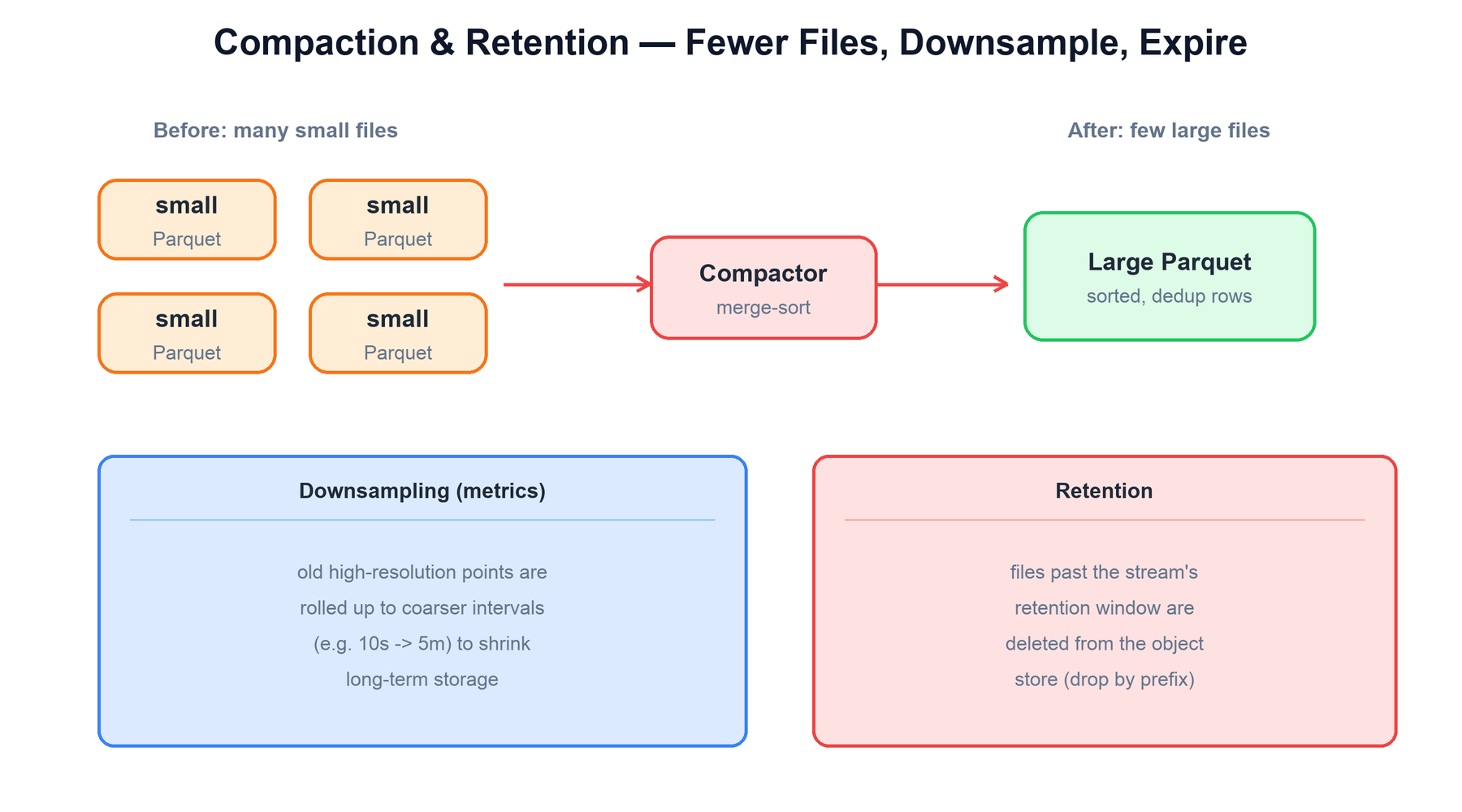
The compactor does three jobs:
| Job | What it does |
|---|---|
| Merge | Reads many small Parquet files for a partition, merge-sorts their rows, deduplicates, and writes one larger, well-ordered Parquet file. Fewer files means fewer object-store requests and tighter min/max ranges, so reads get faster. |
| Downsample | For metric streams, old high-resolution samples are rolled up to coarser intervals (for example 10-second points aggregated to 5-minute points). Recent data stays fine-grained; long-term data shrinks dramatically. |
| Retention | Files older than the stream's retention window are deleted from the object store and de-registered from the metadata store. Because partitions are time-prefixed, expiry is a cheap prefix delete — no row-by-row scanning. |
All three operations are rewrite-and-replace: the compactor writes new files, updates the metadata store to point at them, and then removes the superseded files. Queriers always read whatever the metadata store currently lists, so compaction is invisible to in-flight queries and never blocks ingestion.
on compaction for (stream, partition):
  small = metadata.files(stream, partition, max_size = SMALL)
  if len(small) < MIN_TO_MERGE: return
  merged = merge_sort_dedup(small)            # one larger file
  object_store.put(merged.key, merged)
  metadata.register_file(merged.key, merged.stats)
  metadata.deregister(small)                  # atomic swap in catalog
  object_store.delete(small)                  # reclaim space

on retention sweep:
  for f in metadata.files(stream):
    if f.max_ts < now - stream.retention:
      metadata.deregister(f); object_store.delete(f)
9. Summary
The whole system is built from a few reinforcing ideas:
| Concern | Mechanism |
|---|---|
| Where does data live? | Compressed columnar Parquet on an object store — the only required durable store. The metadata store holds just the catalog. |
| How is it organized? | Organizations contain typed streams (logs/metrics/traces); each stream is partitioned by time plus optional partition keys. |
| How does ingest stay fast? | Append to WAL, ack, buffer in memory, then flush asynchronously to Parquet. Schema is inferred on ingest, never declared. |
| How are reads so cheap? | Layered pruning — partition prefixes, file min/max stats, bloom filters, inverted index — drops files on metadata alone, then reads only the needed columns. |
| How does it execute? | SQL/PromQL planned by DataFusion, scattered across stateless queriers, executed on Arrow batches, gathered at the end. |
| How is storage reclaimed? | The compactor merges small files, downsamples old metrics, and deletes expired partitions by prefix — all rewrite-and-replace in the catalog. |
| How does it scale? | Roles are stateless; add ingesters for write load, queriers for read load. Data and catalog are untouched. |