Designing a Petabyte-Scale Data Pipeline with Strong SLAs
A system design interview guide to moving petabytes through batch and streaming stages that land correct, complete, and on time — where the hard requirement is not throughput but the freshness and quality guarantee attached to the output.
Moving a petabyte is, by now, a solved problem: throw a distributed engine and enough machines at it and the bytes will flow. What makes a petabyte pipeline hard is the promise wrapped around it — that a dataset will be ready by a deadline, complete, correct, and reproducible, every single day, even when an upstream source is late or a schema changes underneath you. That promise is the SLA, and it is what turns a data pipeline from a script into a system. This guide builds such a pipeline: the batch-versus-streaming split (lambda and kappa), ingestion and partitioning, columnar storage with Parquet, a compute engine (Spark or Flink), orchestration and DAGs, and the reliability machinery — data quality gates, schema evolution, lineage, idempotent reprocessing, backfills, and freshness monitoring — that keeps the SLA honest at petabyte scale.
Contents
1. Requirements & Scope
At this scale the requirements that matter are the guarantees, not the volume. Anyone can process a petabyte; the design is judged on whether the output can be trusted and whether it arrives on time.
- Freshness SLA. Output datasets must be ready by a deadline — daily tables by a certain hour, streaming views within seconds to minutes of the event.
- Correctness & completeness. No silent data loss or duplication; the output reflects all and only the intended input.
- Quality. Data must pass validation — row counts, ranges, referential checks — before it is published to consumers.
- Reproducibility. Re-running a stage on the same input yields the same output (idempotent), so backfills and reprocessing are safe.
- Evolvability. Schemas change over time without breaking downstream consumers or historical data.
- Cost. At petabyte scale, storage and compute dollars are a first-class constraint, not an afterthought.
2. Back-of-the-Envelope
Numbers show which choices are forced by scale — particularly why columnar storage and partition pruning are not optional.
| Quantity | Assumption | Result |
|---|---|---|
| Daily volume | ~1 PB/day ingested | ~12 GB/s sustained average |
| Event rate | ~1 KB events | ~10M+ events/sec on the stream |
| Full-scan cost | read 1 PB at ~10 GB/s aggregate | ~28 hours — scanning everything is a non-starter |
| Partition pruning | query one day of a year | read ~1/365 — minutes, not hours |
| Columnar projection | read 5 of 100 columns | ~20× less I/O than row storage |
| Compression | columnar + zstd on typed data | ~3–10× smaller on disk |
The lesson is stark: a full scan of a petabyte takes over a day, so the entire storage design exists to avoid reading data. Partitioning skips irrelevant files, columnar layout skips irrelevant columns, and statistics skip irrelevant row groups. Every query should touch a tiny fraction of the petabyte — that is the whole game.
3. Key Definitions
A few terms recur throughout and are worth fixing precisely.
| Term | Meaning |
|---|---|
| Batch | Processing bounded chunks (e.g. a day) on a schedule — high throughput, higher latency. |
| Streaming | Processing unbounded events continuously — low latency, harder correctness. |
| Lambda | Two paths: a fast approximate speed layer plus an accurate batch layer, merged at read. |
| Kappa | One streaming path; reprocess history by replaying the log — no separate batch code. |
| Idempotent | Re-running produces the same result — safe to retry and backfill. |
| Backfill | Reprocessing historical partitions, e.g. after a bug fix or a new column. |
| Lineage | The recorded map of which inputs produced which outputs. |
4. Architecture: Lambda & Kappa
The first architectural decision is how to reconcile the need for both low latency and full accuracy. Two canonical patterns answer it.
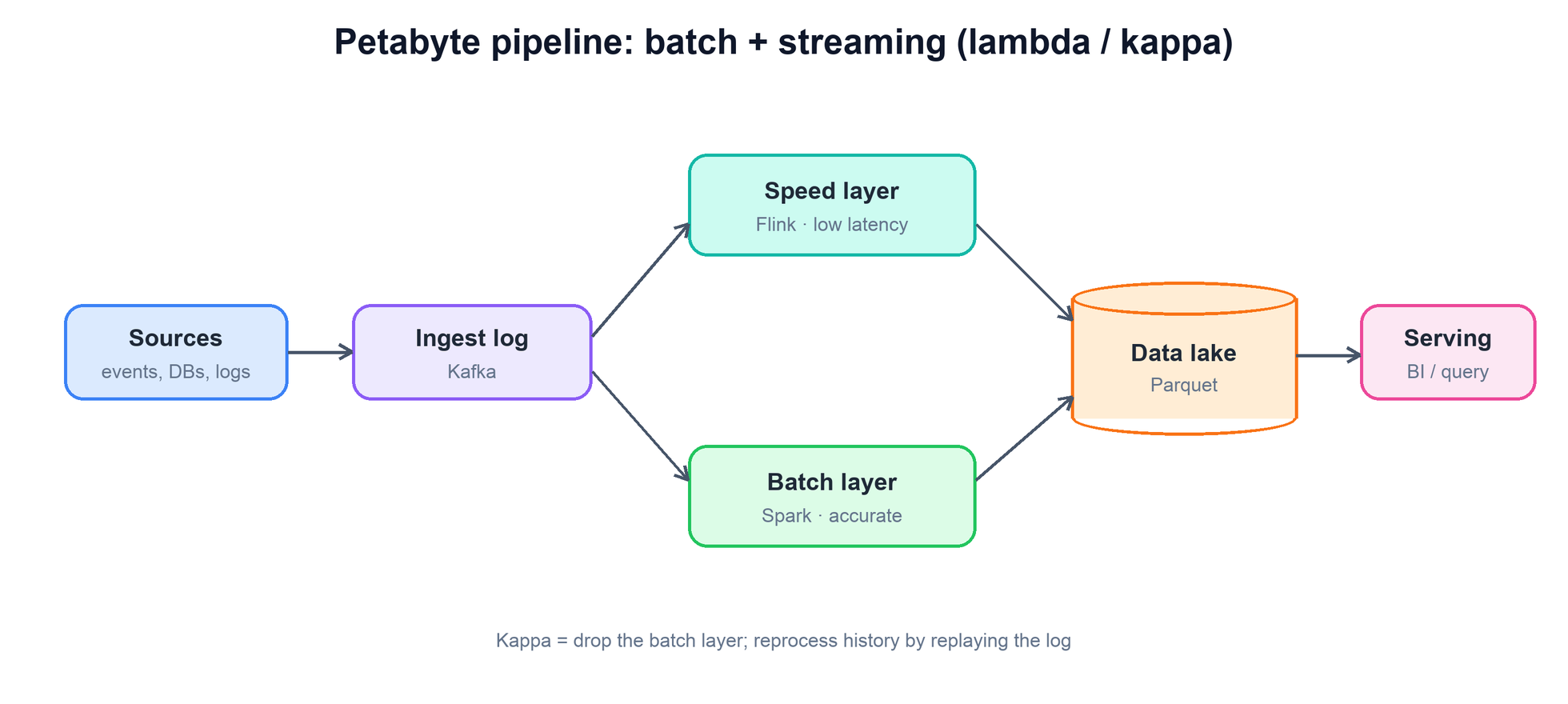
- Lambda architecture. Runs two paths in parallel: a speed layer that processes the stream for immediate, approximate results, and a batch layer that reprocesses the full data for accurate, complete results, with a serving layer merging the two. It delivers both freshness and correctness, but its cost is real: you maintain the same logic twice, in two codebases, and must keep them consistent.
- Kappa architecture. Collapses the two into one streaming path over a durable, replayable log. There is no separate batch code — to reprocess history (a bug fix, a new derived field), you simply replay the log through the same streaming job. It is simpler to maintain, at the cost of needing a stream processor and log retention capable of handling full reprocessing.
The modern lean, especially with an engine that unifies batch and streaming, is toward kappa or a single-engine hybrid: one codebase, replay for history. The durable ingest log (Kafka or equivalent) is the linchpin either way — it decouples producers from consumers, buffers bursts, and, by being replayable, is what makes reprocessing possible at all.
5. Storage, Partitioning & Parquet
Since scanning the whole dataset is impossible, storage is designed entirely around reading as little as possible. Two ideas do the heavy lifting: partitioning and columnar format.
Partitioning lays data out in a directory hierarchy by a coarse key — almost always date, often plus region or another high-selectivity dimension. A query filtered to one day then reads only that day’s files (partition pruning), touching a tiny slice of the lake. The art is choosing a partition granularity that prunes well without creating the small-files problem — millions of tiny files that overwhelm the metadata layer and kill throughput. Daily partitions of compacted, appropriately-sized files are the usual sweet spot.
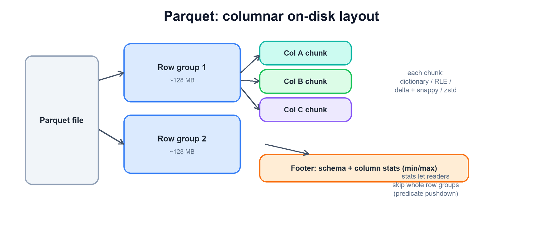
Parquet is the columnar format that makes analytics affordable. Storing each column contiguously means a query reads only the columns it projects — five of a hundred is roughly twenty times less I/O than a row format. Because a column holds values of one type, encoding is highly effective: dictionary encoding for low-cardinality strings, run-length for repeats, delta for sorted numbers, then a general compressor (snappy for speed, zstd for ratio) on top. And the footer’s per-column min/max statistics enable predicate pushdown: a filter like where ts > X lets the reader skip any row group whose max is below X without decompressing it. Partition pruning, column projection, and row-group skipping compound to turn a petabyte lake into a few gigabytes actually read.
6. Compute: Spark vs Flink
The engine executes the transformations across a cluster. The two dominant choices reflect the batch/streaming split, and knowing when to pick which is the point.
| Dimension | Spark | Flink |
|---|---|---|
| Model | Batch-first; streaming as micro-batches. | Streaming-first; batch as a bounded stream. |
| Latency | Seconds (micro-batch interval). | Sub-second, true record-at-a-time. |
| Best for | Large batch ETL, ad-hoc, ML. | Low-latency stateful streaming. |
| State & time | Simpler; less event-time nuance. | Rich event-time, watermarks, large managed state. |
| Exactly-once | Via idempotent/atomic sinks. | Checkpoint + barrier (Chandy-Lamport). |
The mental model: Spark for big, accurate batch; Flink for low-latency, stateful streaming. Both distribute work by partitioning data across executors and running transformations in parallel; the expensive operations are the ones that force a shuffle — joins and group-bys that move data across the network to co-locate keys. Data skew, where one key holds a disproportionate share, creates a straggler task that dominates the whole job’s runtime and is the classic petabyte-scale performance killer. Both engines achieve exactly-once semantics: Flink via distributed checkpoints (barriers snapshot state consistently), Spark via idempotent, atomic writes to the sink so a retried task cannot double-write.
daily_etl:
  raw   = read_parquet("lake/events/date=2026-07-05")  # partition pruning
        .select("user", "event", "ts")                  # column projection
        .filter("ts > cutoff")                          # predicate pushdown
  out   = raw.groupBy("user").agg(...)                  # shuffle: watch for skew
  write_atomic(out, "lake/daily/date=2026-07-05")      # idempotent partition swap
7. Quality, SLAs & Reprocessing
This layer is what upgrades a pipeline into a system with a promise. Each mechanism protects a specific part of the SLA.
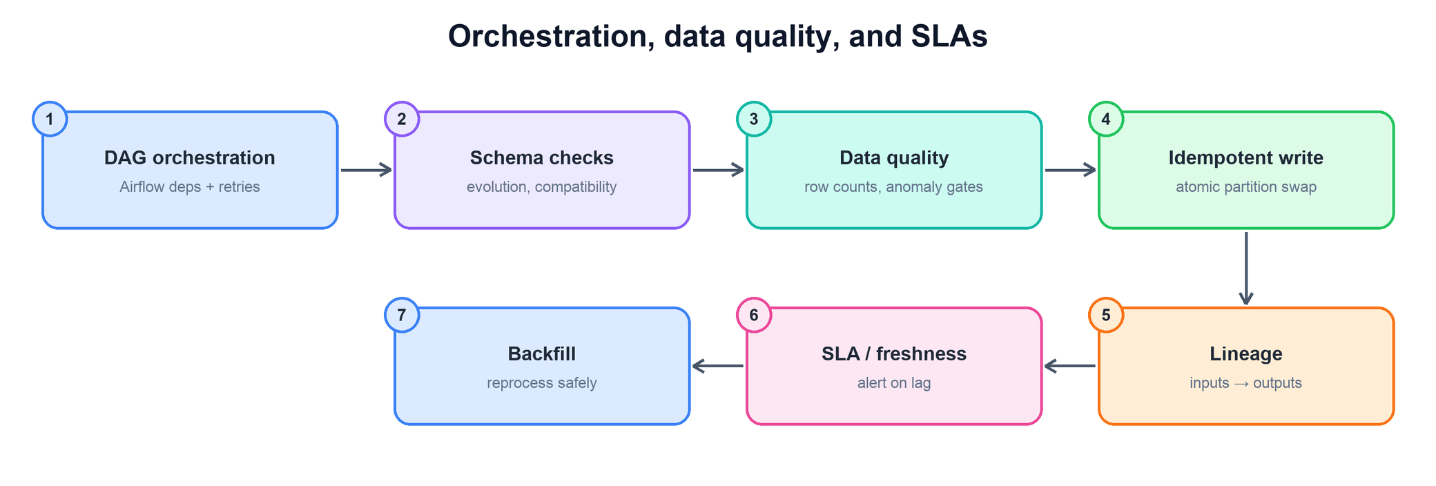
- Orchestration & DAGs. A scheduler (Airflow-style) models the pipeline as a directed acyclic graph of tasks with dependencies, retries, and backfill support, so a stage runs only when its inputs are ready and a transient failure retries automatically.
- Data quality gates. Before publishing, validate: row-count sanity, null and range checks, referential integrity, distribution anomalies. A failed gate blocks the bad partition rather than poisoning downstream consumers — fail the batch, do not ship garbage.
- Schema evolution. Schemas change; a self-describing format plus a schema registry lets you add columns without breaking readers. Enforce backward/forward compatibility rules so old and new data and code interoperate.
- Idempotent reprocessing. Writes are idempotent — typically an atomic swap of a whole partition — so re-running a task produces the same result and a retry never duplicates. This is the property that makes everything else safe.
- Backfills. When logic changes or a bug is fixed, reprocess historical partitions through the same idempotent jobs. Kappa makes this a log replay; either way, idempotency is the prerequisite.
- Lineage. Record which inputs produced which outputs, so you can trace a bad value to its source and know exactly what to reprocess when something is wrong.
- SLA / freshness monitoring. Track per-dataset freshness and completeness and alert when a table is late or a partition is missing — the SLA is only real if you are watching it.
8. Bottlenecks & Tradeoffs
The tensions at petabyte scale are about latency versus correctness, and about the cost of every byte read and stored.
- Latency vs accuracy. Streaming is fresh but must handle late and out-of-order data; batch is complete but delayed. Lambda buys both at the cost of duplicate logic; kappa keeps one path at the cost of a heavier streaming stack.
- Partition granularity. Fine partitions prune better but risk the small-files problem; coarse partitions avoid tiny files but read more per query. Compaction and a daily-ish granularity balance the two.
- Shuffle & skew. Joins and aggregations force network shuffles, and skewed keys create stragglers that dominate runtime. Salting hot keys, broadcast joins for small sides, and good partitioning are the mitigations.
- Cost vs performance. Better compression (zstd) saves storage but costs CPU; more executors finish faster but cost more. At a petabyte these knobs are budget decisions — optimize the columns read and the data stored first, since I/O dominates.
- Schema rigidity vs flexibility. Strict schemas catch errors early but resist change; loose schemas evolve easily but let bad data through. A registry with explicit compatibility rules is the disciplined middle.
9. Summary
A petabyte pipeline is defined by its promise, not its throughput. The storage layer exists to avoid reading data, the compute layer to process what remains in parallel, and the reliability layer to make the output trustworthy and on time.
| Concern | Mechanism |
|---|---|
| Fresh or accurate? | Lambda runs both a speed and batch layer; kappa uses one streaming path with log replay. |
| How do we avoid full scans? | Partition pruning + columnar projection + row-group skipping via Parquet statistics. |
| Why columnar? | Parquet reads only projected columns and compresses typed data 3–10× with encodings. |
| Which engine? | Spark for big accurate batch; Flink for low-latency stateful streaming. |
| How do we get exactly-once? | Flink checkpoints/barriers; Spark idempotent atomic sink writes. |
| How do we make reprocessing safe? | Idempotent, atomic partition swaps — retries and backfills never duplicate. |
| How do we keep data trustworthy? | Quality gates block bad partitions; schema registry governs evolution; lineage traces issues. |
| How do we keep the SLA honest? | DAG orchestration with retries plus freshness/completeness monitoring and alerting. |