Designing a Logs-to-Metrics Real-Time Alerting Pipeline
A system design interview guide to turning a firehose of logs and events into metrics in real time, and paging a human only when something is genuinely wrong — with the false-positive rate kept ruthlessly low.
Every request, error, and state change a service emits shows up first as a log line or an event. On their own these are unstructured and endless; nobody can watch them scroll by. The job of a logs-to-metrics pipeline is to distill that stream into a small number of meaningful metrics — error rate, p99 latency, throughput — and then to alert on those metrics in a way that catches real incidents fast without crying wolf. The hard part is almost never the extraction; it is the alerting. A pipeline that pages on every blip trains its on-call to ignore it, and an ignored alert is worse than no alert at all. This guide builds the pipeline from the stream inward: extraction and windowed aggregation, keeping cardinality under control, the rules engine, thresholds versus anomaly detection, multi-window multi-burn-rate alerting borrowed from Google’s SRE practice, and the dedup, grouping, and flap-damping layers that decide whether a human’s phone actually buzzes.
Contents
1. Requirements & Scope
Before drawing boxes, pin down what the pipeline must do. The interviewer is watching whether you separate the loud requirement (extract metrics) from the subtle one (alert without noise).
- Functional. Consume a high-volume log/event stream; extract numeric metrics via parsing and aggregation; evaluate alerting rules continuously; group and deduplicate firing rules into incidents; route notifications to the right on-call with the right urgency.
- Latency. Detection latency — event to page — should be tens of seconds, not minutes. An alert that arrives ten minutes late has let the incident run ten minutes unattended.
- Low false positives. The primary quality metric is precision of alerts. A high recall (catch everything) that also pages constantly is a failure, because humans stop trusting it.
- Reliability. The alerting path must be more available than the systems it watches. If the pipeline dies silently, every service looks healthy.
- Non-goals. Long-term log storage, full-text search, and forensic drill-down belong to a log store; here we keep only enough to compute and alert on metrics.
2. Back-of-the-Envelope
Rough numbers set the shape of the design and show you can reason about scale. Assume a mid-size fleet emitting a steady event stream.
| Quantity | Assumption | Result |
|---|---|---|
| Event rate | 1M events/sec, ~500 bytes each | ~500 MB/s = ~43 TB/day raw |
| Extraction fan-out | ~20 metrics derived per event on average | ~20M metric updates/sec |
| Active series | metric × bounded tags (service, endpoint, status, region) | target < a few million series |
| Aggregated output | series flushed at 10s resolution | ~few hundred K points/sec — a 100× reduction |
| Alert rules | ~5K rules, each over a handful of windows | evaluated every 10–30s tick |
| Detection budget | ingest + window + evaluate + route | ≤ ~30s end to end |
The headline is the reduction: aggregation collapses tens of millions of per-event updates into a few hundred thousand metric points per second. That collapse is what makes real-time alerting affordable — you evaluate rules over compact aggregates, never over raw logs.
3. Metrics & Rule Definitions
Two definitions carry the whole design: what a metric is, and what an alerting rule is. Getting them precise up front keeps the later layers simple.
A metric extracted from the stream is the familiar time-series tuple: a name, a set of bounded key-value tags, a timestamp, and a value. Metrics come in the usual shapes — a counter for events (requests, errors), a gauge for levels (queue depth), and a histogram for distributions (latency), from which quantiles like p99 are computed.
An alerting rule binds a query over those metrics to a condition, a duration, and a routing decision:
# a rule is data, not code — declarative and version-controlled
rule high_error_rate:
  expr:      rate(errors[5m]) / rate(requests[5m])   # the SLI
  condition: > 0.02                                    # 2% error budget burn
  for:       2m                                        # must persist to fire
  labels:    { severity: page, team: checkout }
group_by: [service, region] # dedup dimension| Field | Purpose |
|---|---|
expr | The metric query — a rate, ratio, or quantile computed over a window. |
condition | The threshold or anomaly test that decides “bad.” |
for | How long the condition must hold before firing — the first line of noise defense. |
labels | Severity and routing metadata attached to the resulting alert. |
group_by | The dimensions along which firing instances collapse into one incident. |
4. High-Level Architecture
The pipeline is a directed flow from raw stream to human. Each stage does one job, and the noise-reduction stages sit deliberately near the end, after the metric has already been computed.
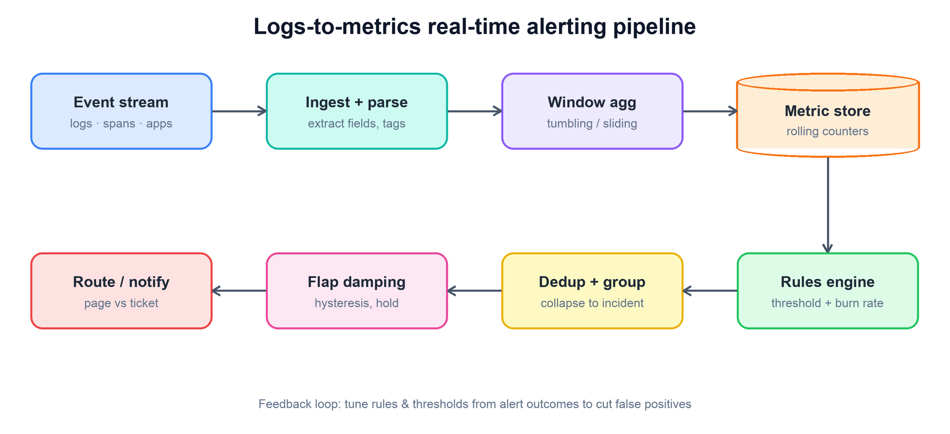
- Event stream. A durable, partitioned log (Kafka-style) buffers the firehose and lets consumers scale out and replay. Partitioning by a stable key keeps a given series’ events on one consumer.
- Ingest + parse. Stateless workers parse each event, extract fields, and emit metric updates with bounded tags. This layer scales horizontally with the stream.
- Window aggregation. Updates are folded into time windows per series — the step that turns millions of events into compact points.
- Metric store. A short-retention time-series buffer holds recent aggregates for rule evaluation; long history can spill to a full TSDB.
- Rules engine. Evaluates each rule on every tick against the store, producing candidate alerts.
- Dedup, flap damping, routing. Collapse duplicates, suppress flapping, and deliver to the right on-call at the right urgency.
5. Windowing & Cardinality
Aggregation happens over windows of time, and the choice of window shape trades latency against smoothness. Two shapes dominate.
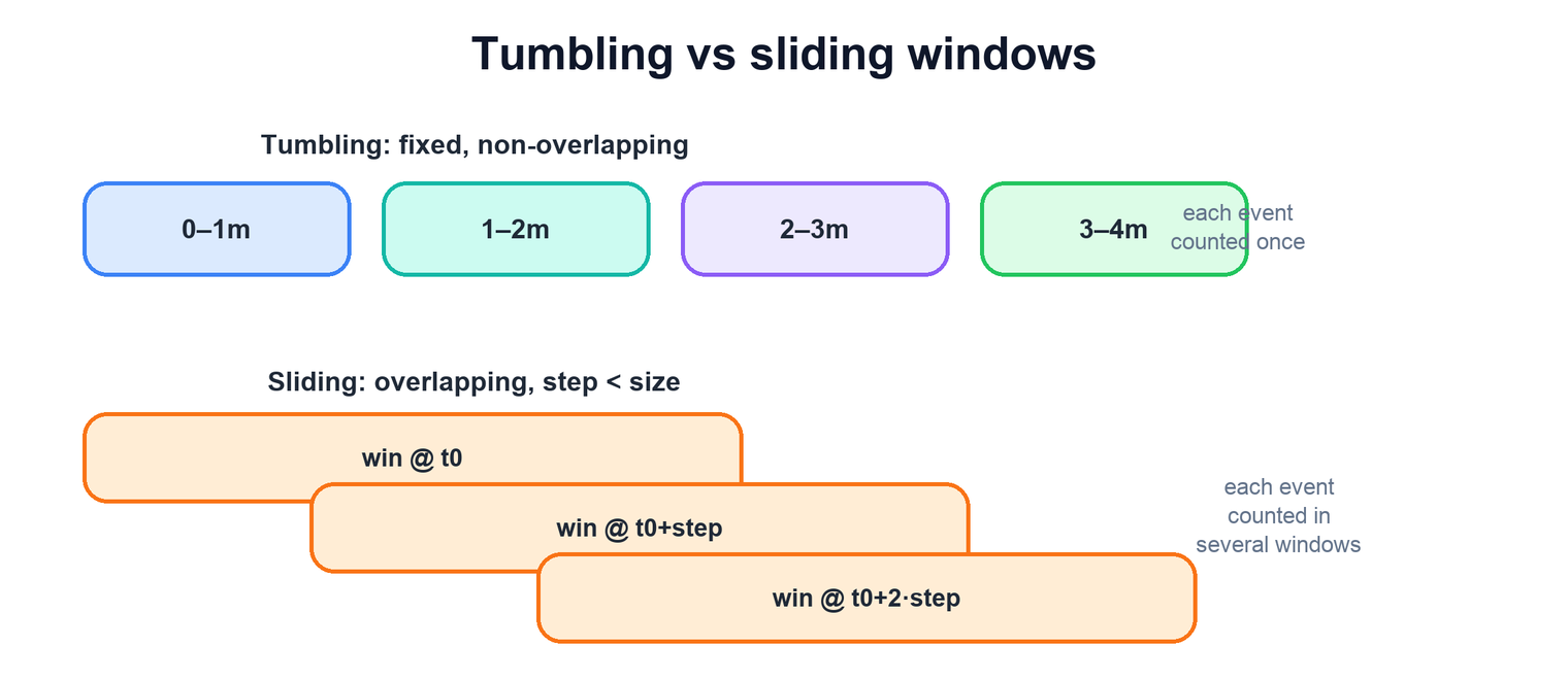
- Tumbling windows are fixed and non-overlapping — the classic “per-minute count.” Cheap and exact, but the metric only updates once per window, adding up to a full window of detection latency.
- Sliding windows overlap, advancing by a small step. They update more often and smooth out edge effects, at the cost of holding more state and doing more work per event.
Late and out-of-order events are unavoidable in a distributed stream, so aggregation is driven by event time with a watermark — a moving estimate of “we have probably seen everything up to time T” — that decides when a window is complete enough to emit, plus a small grace period for stragglers.
on event(e):
  ts = e.event_time                          # event time, not arrival time
  if ts < watermark - grace:
    drop_or_side_output(e)                    # too late; don't corrupt closed windows
    return
  for w in windows_covering(ts):             # 1 tumbling, several sliding
    agg[w][series(e)].update(e.value)
  advance_watermark()
  emit_windows_below(watermark)              # flush complete windows
Cardinality control is the make-or-break constraint. Every distinct combination of metric name and tag values is a separate series the pipeline must hold state for, and the count multiplies across tags. A tag with unbounded values — user id, request id, raw URL with query string — mints a new series forever and exhausts memory. The defenses: allow only a curated set of low-cardinality tags; normalize high-variety fields (bucket URLs to route templates, strip ids); and enforce a hard per-metric series limit that sheds or aggregates the overflow rather than letting a bad label take the pipeline down.
6. Thresholds, Anomalies & Burn Rate
Given clean metrics, the alerting logic decides what is worth a page. There are two families of condition, and a structural pattern that makes either one trustworthy.
Static thresholds compare a metric to a fixed line — error rate above 2%, latency above 500 ms. They are simple, explainable, and easy to reason about, but brittle: a good line for peak traffic pages constantly at 3 a.m., and a line for quiet hours misses a daytime regression.
Anomaly detection compares a metric to its own expected behavior — a forecast from history, or a band of several standard deviations around a seasonal baseline. It adapts to daily and weekly cycles and catches “weird for right now” that a static line misses, but it is harder to explain, needs training data, and can be fooled by a slow drift it learns to accept. In practice teams use static thresholds for the things with a real SLO and reserve anomaly detection for shapes no fixed line captures.
The pattern that makes alerting precise and fast is multi-window, multi-burn-rate alerting, from the Google SRE workbook. Instead of one threshold, you alert on how fast the error budget is burning, measured over several windows at once.
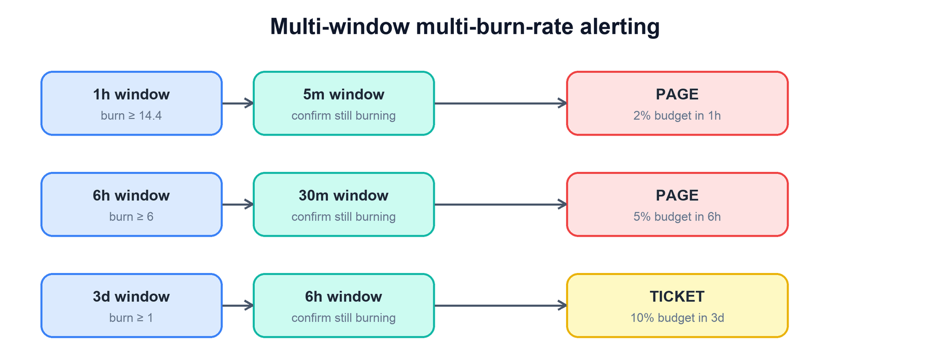
The burn rate is how many times faster than sustainable you are consuming the error budget. A 30-day 99.9% SLO burned at 1× lasts exactly the month; at 14.4× it would be gone in about two days — so a 14.4× burn over one hour means you have already spent 2% of the whole month’s budget in that hour, and that warrants an immediate page. The two-window trick is what kills noise: the long window gives sensitivity, and the short window acts as a reset — the alert only fires while the short window also shows the burn, so it clears quickly once the incident is over instead of hanging around.
| Severity | Long / short window | Burn rate | Budget consumed |
|---|---|---|---|
| Page (fast) | 1h / 5m | 14.4× | 2% in 1 hour |
| Page (slow) | 6h / 30m | 6× | 5% in 6 hours |
| Ticket | 3d / 6h | 1× | 10% in 3 days |
function fires(rule, now):
  for (long, short, threshold) in rule.burn_windows:
    lb = burn_rate(rule.sli, long,  now)   # budget burn over long window
    sb = burn_rate(rule.sli, short, now)   # and over short window
    if lb >= threshold and sb >= threshold: # both must agree
      return true                          # short window makes it reset fast
return falsefor duration so momentary spikes self-heal, multi-window burn rate so you page on budget burn rather than instantaneous value, the short-window confirm so alerts clear when the incident ends, and grouping plus flap damping downstream. Precision comes from the stack, not one clever number.7. Dedup, Grouping & Flap Damping
A rule that fires is not yet a page. Between firing and the phone buzzing sit the layers that turn many correlated signals into one actionable notification — the difference between a useful alert and an alert storm.
- Deduplication. The same rule firing on the same target every tick is one alert, not hundreds. Alerts are keyed by rule plus
group_bylabels, and a repeat within an active window just refreshes the existing one. - Grouping. When a shared dependency fails, dozens of rules fire at once. Grouping collapses them by a common dimension — region, cluster, service — into a single incident notification, so on-call gets one page describing the blast radius instead of forty.
- Flap damping. A metric hovering at the threshold flips fire/resolve/fire endlessly. Hysteresis fixes it: fire above a high line, resolve only below a lower one, and hold a resolved alert for a cool-down before declaring it truly over.
- Routing & escalation. The grouped, damped alert is routed by its labels to the owning team’s on-call, at page or ticket urgency, with escalation if unacknowledged and silences for known maintenance.
on rule_fires(alert):
  key = (alert.rule, alert.group_labels)     # dedup identity
  if active[key] and not cooled_down(key):
    active[key].refresh(); return            # dedup: same incident
  group = correlate(alert)                    # collapse related fires
  if flapping(key):
    hold(key); return                         # hysteresis + cool-down
  route(group, urgency=alert.severity)        # page vs ticket
Closing the loop, alert outcomes feed back into the rules. Every page that a human marks “not actionable” is evidence to raise a threshold, lengthen a for, or add a grouping dimension. Treating false positives as bugs to be fixed — not noise to be tolerated — is what keeps the pipeline trusted over time.
8. Bottlenecks & Tradeoffs
The interesting failure modes cluster around state, latency, and the perennial tension between catching everything and paging too much.
- Cardinality vs granularity. More tags mean richer slicing but combinatorial series growth. The trade is resolved by curating tags and normalizing high-variety fields, accepting coarser granularity to stay within a series budget.
- Latency vs stability. Short windows and small watermark grace detect faster but emit noisier, more revisable results; longer windows are stable but slow. Burn-rate tiers let you have both — fast pages for severe burns, slow tickets for gradual ones.
- Precision vs recall. Every noise defense that raises precision (longer
for, higher burn threshold) risks missing a genuine slow-burn issue. The multi-tier design is precisely a way to buy recall on the slow path without sacrificing precision on the fast one. - Pipeline availability. The alerting path must outlive what it watches. That means running it in a separate failure domain, monitoring the monitor with a dead-man’s switch (a heartbeat alert that fires if the pipeline goes quiet), and degrading gracefully when the stream lags.
- Stateful aggregation. Windowed state is the scaling limit; it must be partitioned by series key, checkpointed for recovery, and bounded so a cardinality spike cannot exhaust memory.
9. Summary
A logs-to-metrics alerting pipeline earns its keep not by extracting metrics — that part is easy — but by paging a human only when it matters. Every layer past aggregation exists to raise precision without losing the incidents that count.
| Concern | Mechanism |
|---|---|
| How do we cut the firehose down? | Windowed aggregation collapses per-event updates into compact series — a large reduction. |
| How do we aggregate correctly? | Event-time windows (tumbling or sliding) driven by watermarks, with a grace period for late data. |
| What is the dominant scaling limit? | Cardinality — curate bounded tags, normalize high-variety fields, cap series per metric. |
| Static line or adaptive? | Thresholds for SLO-backed signals; anomaly detection for seasonal shapes a fixed line misses. |
| How do we page fast yet precisely? | Multi-window multi-burn-rate: long window for sensitivity, short window to confirm and reset. |
| How do we avoid alert storms? | Dedup by rule+labels, group correlated fires into one incident, damp flapping with hysteresis. |
| How do we keep it trusted? | Feed alert outcomes back to tune rules; treat every false positive as a bug to fix. |
| How do we keep the monitor alive? | Separate failure domain plus a dead-man’s switch that fires if the pipeline goes silent. |