Designing a Distributed Log Search Engine
A system design interview guide to building a log search engine that ingests exabytes, indexes them for near-real-time search, and answers a query across a fleet in seconds — the machinery behind systems like Elasticsearch, OpenSearch, and Loki.
Logs are the highest-volume, most detailed telemetry a system produces, and searching them is deceptively hard: you want to type a free-text query and instantly find the handful of relevant lines out of trillions, spanning data from seconds ago to years ago. That requires two ideas working together — an inverted index that maps terms to the documents containing them, so a search never scans everything, and a distributed, tiered architecture that shards the index across many machines and moves aging data down a hot–warm–cold ladder onto cheap object storage. This guide builds that engine: the index model borrowed from Lucene, sharding and time-partitioning, the tiered storage that makes exabytes affordable, and the scatter-gather query path that turns a query string into a plan executed across shards.
Contents
1. Requirements & Scope
The engine ingests a firehose of log lines and serves search over them. Pin down the requirements.
- Functional. Ingest structured and unstructured log lines; full-text and field search with filters (service, level, time range); aggregations (counts, histograms over time); and results ranked or ordered by time.
- Near-real-time. A log line should be searchable within seconds of being emitted — incidents happen now, not after a batch job.
- Scale. Exabytes of retained data, millions of lines per second ingested, queries fanning across thousands of shards.
- Query latency. Interactive queries on recent data in well under a second; historical queries over cold data in seconds.
- Cost. Retaining exabytes on hot storage is impossible; the design must tier aggressively onto cheap object storage while keeping old data searchable.
- Custom query language. A DSL that expresses filters, full-text, and aggregations, compiled to a plan executed across shards.
2. Back-of-the-Envelope Estimates
Assume 5,000,000 log lines/second at 500 bytes each, retained 13 months.
| Quantity | Estimate | Volume math |
|---|---|---|
| Ingest | ~2.5 GB/s raw | 5M lines/s × 500 B = 2.5×10⁹ B/s. |
| Daily volume | ~216 TB/day raw | 2.5 GB/s × 86,400 s. |
| Retained (compressed) | ~20–30 PB | 216 TB/day × ~395 days × ~1 replica ÷ ~4× compression → tens of PB. |
| Index overhead | +10–100% of raw | Full inverted index can equal or exceed raw size — hence index only high-value fields. |
| Hot tier | ~1–2 days on SSD | Most queries hit recent data; keep only days hot, age the rest to warm/cold object storage. |
The math drives the architecture directly: index overhead can rival the raw data, so you cannot fully index everything; and retaining PBs is only affordable on object storage, so the design must keep cold data searchable from S3-class storage rather than local disk.
3. The Index Model & Segments
The core data structure is the inverted index, the same one Lucene provides beneath Elasticsearch and OpenSearch. Instead of storing documents and scanning them, it stores, for every term, the list of documents that contain it — a postings list. A search for level:ERROR becomes an O(1) dictionary lookup returning the exact matching documents, and combining terms is a fast intersection or union of postings lists.
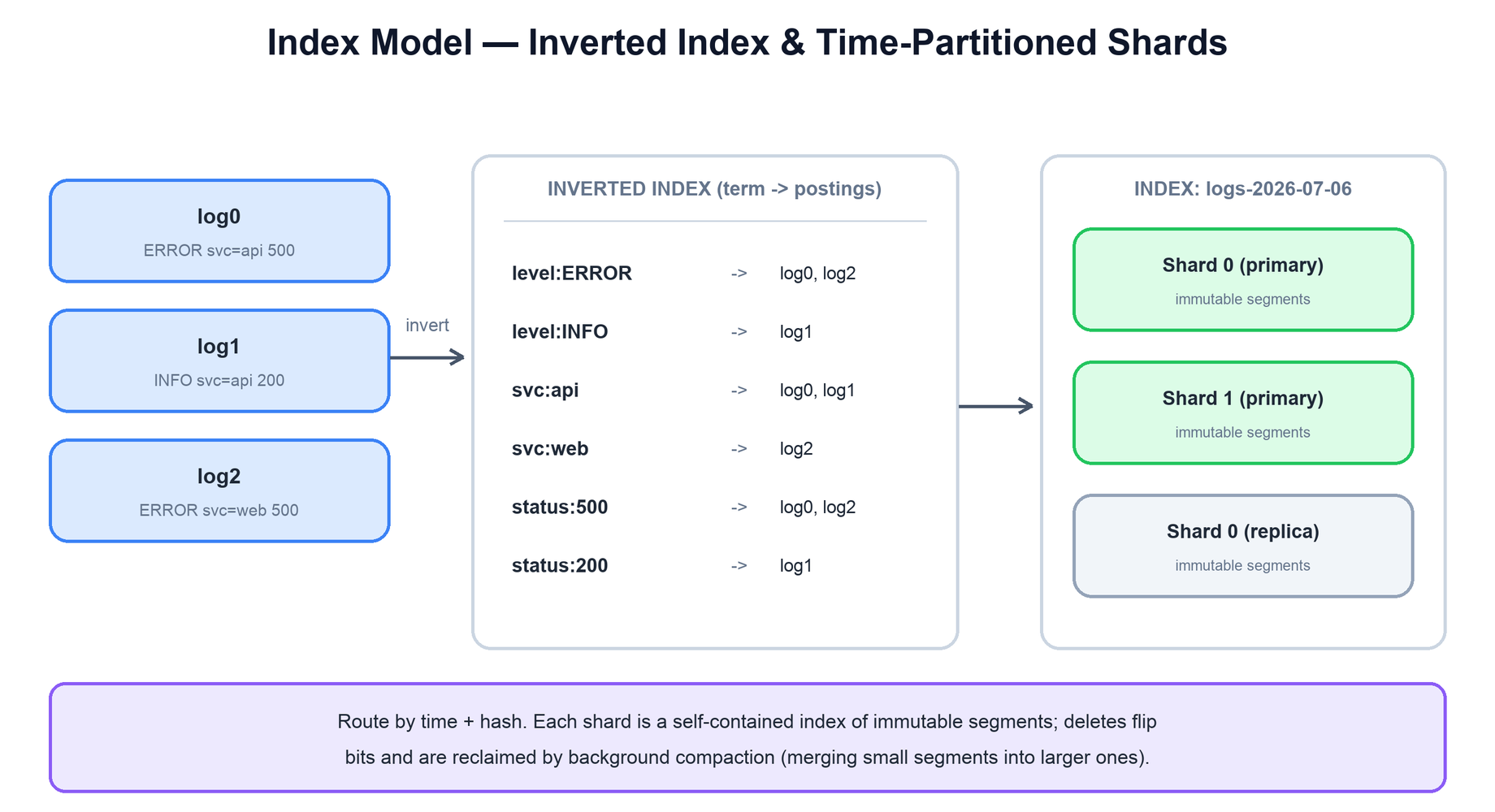
status:500 or svc:api) to the postings list of documents containing it. An index is time-partitioned (one per day), split into shards for scale, and each shard is a set of immutable segments.Three properties of the Lucene model matter for the design:
- Segments are immutable. New documents are buffered and periodically flushed into a new, immutable segment (a self-contained mini-index). Immutability makes writes append-only and reads lock-free, but it means deletes only mark tombstones and updates write a new version — space is reclaimed later by merging.
- Near-real-time via refresh. A flushed segment sits in the OS file cache and becomes searchable on the next refresh (typically ~1s) — without a durable commit — which is how new logs become searchable within seconds. A separate write-ahead log (the translog) provides durability before the expensive commit.
- Beyond text. Alongside postings, segments store doc values (a columnar layout for sorting and aggregation) and numeric points (BKD trees for range queries like time filters). Aggregations and time-range filters use these, not the inverted index.
# inverted index: term -> postings list
"level:ERROR"  -> [log0, log2, log7, ...]
"svc:api"      -> [log0, log1, log5, ...]
"status:500"   -> [log0, log2, ...]

# query "ERROR from api" = intersect the postings lists
match = postings["level:ERROR"] & postings["svc:api"]   # fast set intersection
4. Sharding & Time-Partitioned Indices
One machine cannot hold exabytes, so the index is partitioned two ways.
Time-partitioned indices
Logs are overwhelmingly queried by recent time, so the primary partitioning is by time: create a new index per day (or hour), e.g. logs-2026-07-06. This is the highest-leverage decision in the design because it makes two things trivial. Queries with a time range touch only the relevant indices and skip the rest entirely (partition pruning). And retention/tiering is a whole-index operation — to expire or move old data you drop or migrate an entire old index, with no per-document deletes.
Shards within an index
Each time index is split into shards — each shard being an independent Lucene index — so ingest and search scale horizontally. A document routes to a shard by hashing a routing key (default the doc id, or a tenant id to co-locate a tenant’s data). Each shard has replicas on other nodes for availability and read throughput. Shard count is a real tradeoff: too few and you cannot parallelize or grow; too many and per-shard overhead and query fan-out costs dominate (the “oversharding” problem).
| Partitioning | By | Buys |
|---|---|---|
| Time-partitioned index | Event time (per day/hour) | Prune by time; tier/expire whole indices cheaply. |
| Shard | Hash of routing key | Horizontal ingest & search scale; parallelism. |
| Replica | Copy of a shard | Availability + read throughput. |
5. Ingest & Tiered Storage
Affordability at exabyte scale comes from moving data down a cost/latency ladder as it ages, since query frequency drops sharply with age.
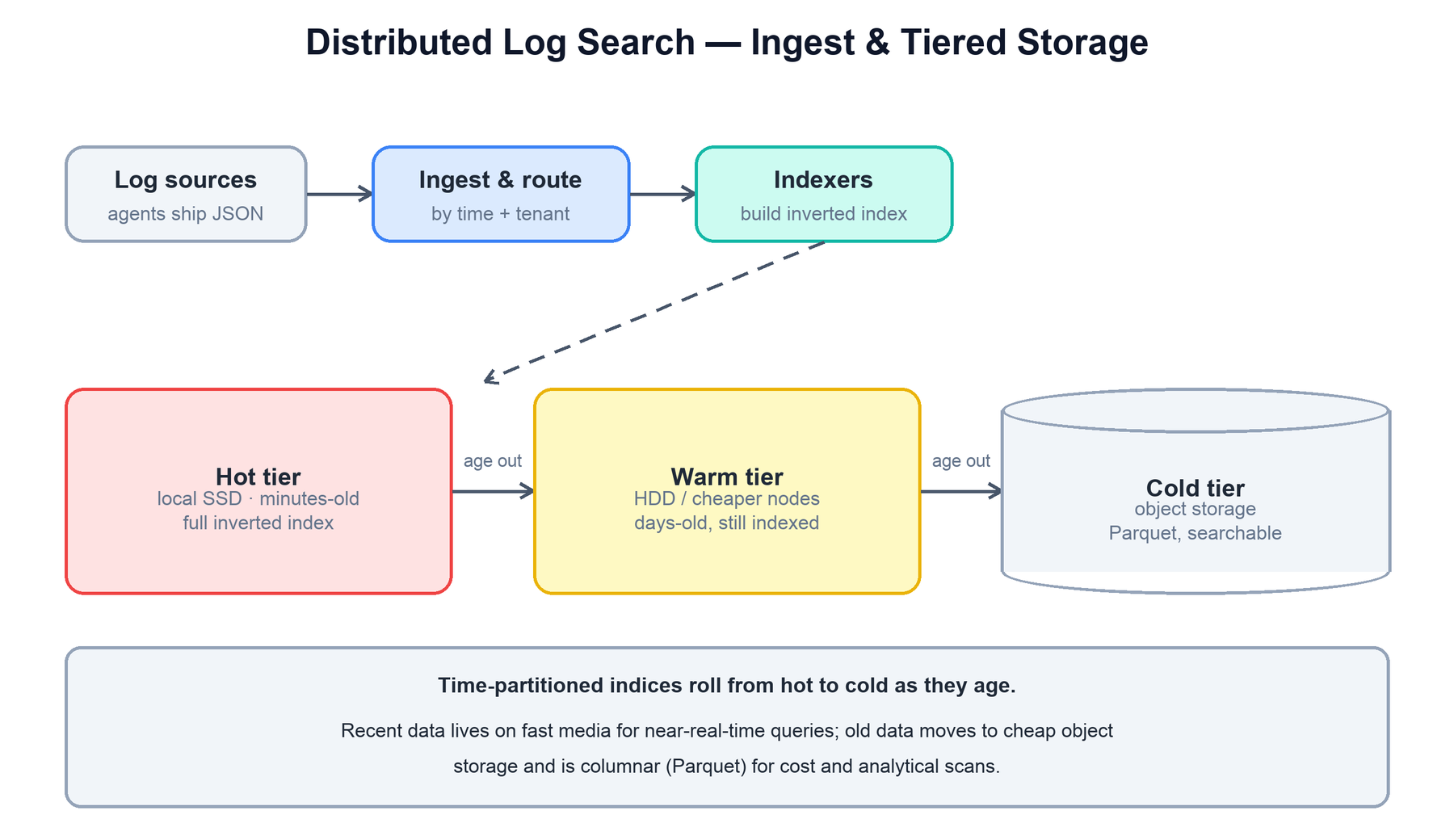
- Hot. Recent indices on local SSD, fully indexed, serving near-real-time ingest and interactive queries. Small, fast, expensive — kept to days.
- Warm. Older indices moved to cheaper nodes (more storage, less CPU/RAM), still indexed and searchable but not receiving writes. Read-only and often force-merged into fewer segments for query efficiency.
- Cold / frozen. Old indices whose data lives on object storage (S3-class). The node keeps only lightweight metadata and fetches blocks on demand — higher query latency but a fraction of the cost. This searchable-snapshot pattern is what makes retaining exabytes possible; storage cost decouples from compute.
Data moves down the ladder automatically by index age via a lifecycle policy, and is eventually deleted when it exceeds retention. Because everything is a whole-index operation, tiering is cheap and does not touch individual documents.
6. Query Execution & Scatter-Gather
A query is expressed in a DSL and executed in three phases: parse the query string into an AST, plan it (resolve which indices and shards it touches, prune by time and tenant, choose whether to use the inverted index, doc values, or points), and execute it across shards with scatter-gather.
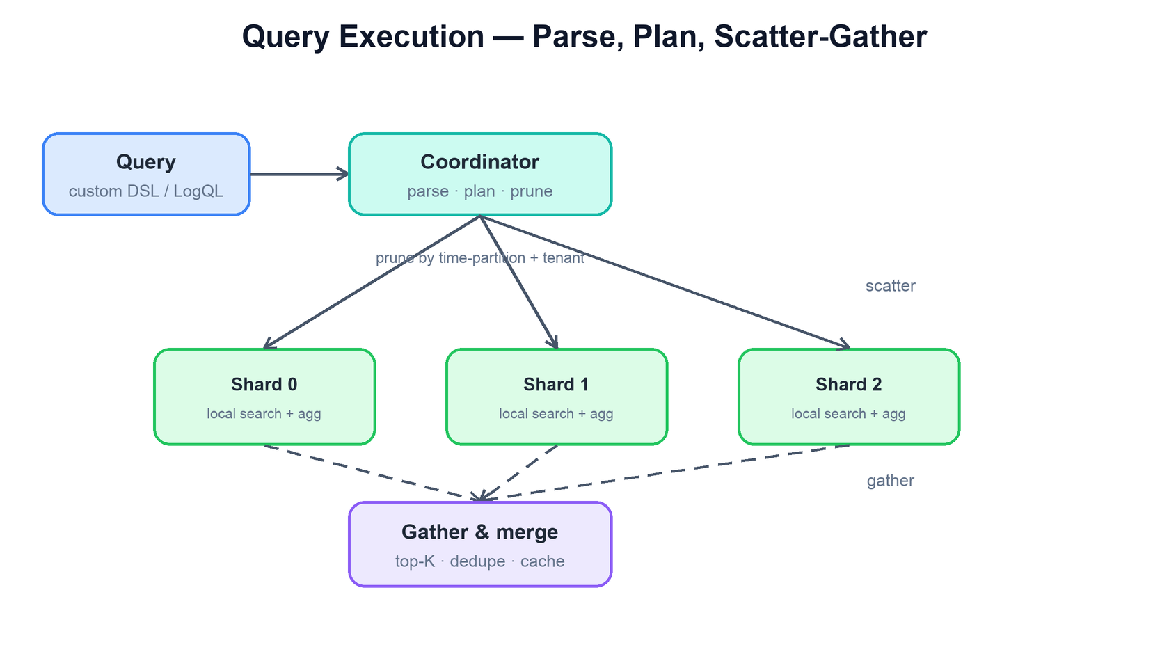
The execution model is scatter-gather: a coordinator fans the query to every relevant shard, each shard runs the query against its local segments and returns a partial result (top-K hits, or partial aggregation), and the coordinator merges the partials into the final answer. Two optimizations are essential at scale. Pruning — using the time range to skip whole indices and shards — is what keeps a “last 15 minutes” query from touching a year of data. And caching — of filter results, of frequently hit shards, of aggregation results — absorbs repeated dashboard queries. A two-phase approach (query phase returns just doc ids + scores; fetch phase retrieves the full documents only for the final winners) avoids shipping large documents from shards that will not make the top-K.
function search(dsl, time_range):
  ast     = parse(dsl)                          # -> filters, full-text, aggs
  shards  = plan(ast, time_range)               # prune by time + tenant
  partials = scatter(shards, ast)               # each shard searches locally
  return gather(partials, ast.agg)              # merge top-K / aggregations
7. Columnar Analytics, Caching & Compaction
Three supporting mechanisms round out the engine.
Columnar for analytics. Full-text search wants an inverted index, but analytical queries (“count errors per service per hour over a month”) want to scan a few columns over vast rows — exactly what a columnar format like Parquet excels at. So cold data is stored columnar on object storage: cheap, compressible, and fast to scan for aggregations. Modern systems increasingly split the two — an inverted index for search on hot data, columnar files for analytics on cold data — rather than paying full indexing cost forever.
Caching. Query patterns are heavily repeated (dashboards refresh, alerts re-run), so cache aggressively: OS page cache for hot segments, a query/filter cache for reused predicates, and a results cache for identical dashboard queries. Caching is often the difference between a sub-second and a multi-second dashboard.
Compaction / merging. Because segments are immutable and small ones accumulate, background merging rewrites many small segments into fewer large ones. This bounds the number of segments a query must visit (search cost grows with segment count), and is the only time tombstoned/deleted documents are physically reclaimed. On warm data, an explicit force-merge into a single segment maximizes read efficiency since no more writes are coming.
8. Bottlenecks & Tradeoffs
- Index everything vs index selectively. A full inverted index can exceed the raw data in size. Indexing only high-value fields (and storing the rest for scan/columnar) trades some query flexibility for a large cost saving.
- Shard count. Too few shards caps parallelism and growth; too many multiplies overhead and query fan-out. Size shards to a target (e.g. tens of GB each) and use time-partitioning to bound their lifetime.
- Refresh interval vs cost. Frequent refresh gives lower search latency for new data but creates many small segments and more merge work. Relax it for high-ingest, low-freshness workloads.
- Hot storage cost vs query latency. Keeping more data hot is faster but far more expensive; tiering saves money at the cost of higher latency on old data. Tune the ladder to the query-age distribution.
- Write vs query contention. Heavy ingest and heavy search compete for the same nodes. Separating write (hot, indexing) from read (warm/cold, query) roles keeps a query storm from stalling ingestion.
9. Summary
A distributed log search engine combines the inverted index (search as lookup, not scan) with time-partitioned, sharded, tiered storage (recent data hot and fully indexed, old data cheap on object storage), executed with scatter-gather across shards.
| Concern | Mechanism |
|---|---|
| How do we search without scanning? | Inverted index: term → postings list; combine terms by set intersection/union. |
| How are writes made cheap & safe? | Immutable segments, append-only, with a translog for durability; near-real-time via refresh. |
| How do we scale & prune? | Time-partitioned indices (prune by time) split into hashed shards with replicas. |
| How do we afford exabytes? | Hot/warm/cold tiers; cold data searchable from object storage (searchable snapshots). |
| How do we run a query? | Parse → plan (prune) → scatter to shards → gather & merge; cache repeated queries. |
| How do we serve analytics cheaply? | Columnar (Parquet) for cold data; scan a few columns over many rows. |
| How do we keep queries fast over time? | Background compaction merges small segments and reclaims deleted space. |