Designing a Distributed Tracing System
A system design interview guide to building a tracing system that follows one request across dozens of services, so you can see exactly where the latency and errors went — the machinery behind Dapper, Jaeger, Tempo, and OpenTelemetry.
In a microservice architecture a single user request fans out across dozens of services, and when it is slow or fails, metrics tell you that something is wrong and logs tell you what happened on one machine — but neither tells you where, across the whole call path, the time went. Distributed tracing answers that by stitching together the work done for one request into a single causal timeline. The idea, popularized by Google’s Dapper paper and now standardized by OpenTelemetry, is to tag each request with a trace id, propagate it across every service hop, and have each service emit timed spans that a backend reassembles into a tree. This guide builds that system: the trace and span model, context propagation over the wire, the collector pipeline, the all-important sampling decision (head vs tail), storage at petabyte scale, and trace assembly into waterfalls and dependency graphs.
Contents
1. Requirements & Scope
The system captures the end-to-end path of requests and lets an engineer inspect any one of them. Pin down the requirements.
- Functional. Capture spans across all services for a request; reassemble them into a trace (a tree/waterfall); let users search traces by attributes (service, latency, error, trace id) and view a single trace’s timeline; derive a service dependency graph and latency breakdowns.
- Low overhead. Instrumentation must add negligible latency and CPU to the traced services — tracing that slows production is worse than no tracing.
- Scale. Millions of spans per second raw; petabytes of trace data if unsampled — so sampling is a core requirement, not an add-on.
- Correlation. Traces must link to logs and metrics via shared ids so investigation crosses pillars.
- Freshness. A trace should be viewable within seconds of the request completing.
2. Back-of-the-Envelope Estimates
Assume 1,000,000 requests/second, each producing 20 spans across services, each span ~1 KB.
| Quantity | Estimate | Volume math |
|---|---|---|
| Raw spans | ~20M spans/s | 1M req/s × 20 spans. |
| Raw volume (unsampled) | ~20 GB/s → ~1.7 PB/day | 20M spans/s × 1 KB × 86,400 s — infeasible to store fully. |
| After 1% sampling | ~200k spans/s → ~17 TB/day | Sampling is what turns petabytes into a manageable stream. |
| Retained (7 days) | ~120 TB | 17 TB/day × 7; object storage keeps this cheap. |
| Trace assembly window | seconds | Spans of one trace arrive within seconds; assembly and tail-sampling buffer over that window. |
The dominant conclusion is unavoidable: at 1.7 PB/day raw, you cannot store every trace, so sampling is the central design decision — and where you make it (at the source vs after buffering the whole trace) shapes the entire pipeline.
3. The Trace & Span Model
The data model is small and worth stating precisely. A span is a single named, timed unit of work — one operation in one service. A trace is the collection of all spans for one request, linked into a tree by parent references.
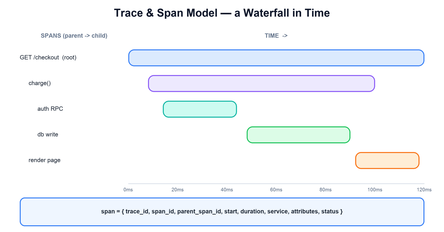
GET /checkout) spans the whole request; child spans (charge, auth RPC, db write, render) nest under it with their own start times and durations. Each span carries a trace_id, span_id, parent_span_id, timing, and attributes.Each span carries:
trace_id— the same for every span in the request; the join key for the whole trace.span_id— unique to this span.parent_span_id— the span that caused this one; null for the root. This is what builds the tree.- start time & duration — the timing that makes the waterfall.
- service / operation name, status, and attributes — tags (http method, db statement, error) and events for detail.
The parent/child links are the essence: the backend does not need spans to arrive in order or together — it just needs each span’s trace_id and parent_span_id to reconstruct the tree later. That decoupling is what lets spans stream in independently from many services.
4. Instrumentation & Context Propagation
The hard part of tracing is not recording a span — it is making sure every service in the request shares the same trace_id. That is context propagation, and it is what turns per-service spans into one coherent trace.
How it works. When a request enters the system, the first service either reads an incoming trace context or starts a new trace. On every outbound call it injects the current trace context into the request — for HTTP, the W3C Trace Context standard puts it in the traceparent header. The next service extracts it, continues the same trace, and repeats. This propagation must cover every hop, including the tricky ones: async work, thread pools, and message queues (where the context rides in message metadata rather than an HTTP header).
# W3C traceparent header format
traceparent: 00-4bf92f3577b34da6a3ce929d0e0e4736-00f067aa0ba902b7-01
             |  |                                |                |
           version   trace-id (16 bytes)      parent span-id   flags (sampled)

# each hop: extract -> start child span -> inject into next call
ctx  = extract(request.headers)                # continue the trace
span = tracer.start_span("db.query", parent=ctx)
inject(outbound.headers, span.context())       # propagate downstream
Instrumentation — the code that starts/ends spans and does inject/extract — comes in two forms: automatic (agents and libraries that instrument common frameworks with no code changes) and manual (developers adding spans around important custom logic). OpenTelemetry provides both a vendor-neutral API/SDK and the propagation standard, which is why it has become the default: instrument once, and any backend can consume the spans. The flags byte in traceparent also carries the sampled bit, so a head-sampling decision made at the edge is honored by every downstream service.
5. High-Level Architecture
The pipeline moves spans from instrumented services, through a collector that batches and samples, into scalable storage, with a read side that assembles and analyzes traces.
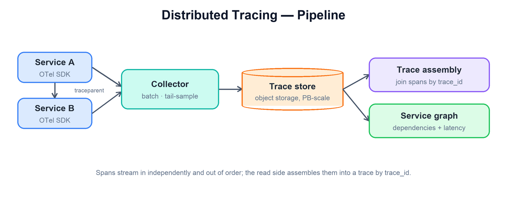
- SDK / agent. In each service, records spans and propagates context with minimal overhead; buffers and exports spans asynchronously so tracing never blocks the request.
- Collector. A tier (often the OpenTelemetry Collector) that receives spans, batches them, enriches them, and — critically — is where tail sampling happens, because it can see all spans of a trace before deciding. It shields storage from load spikes and applies policy centrally.
- Storage. Spans keyed by
trace_idin a store backed by cheap object storage, with a secondary index for search. - Query / UI. Assembles spans into a trace waterfall, supports search by attributes, and computes the service dependency graph.
6. Sampling: Head vs Tail
Since storing every trace is infeasible, you keep a representative and interesting subset. The central choice is when to decide.
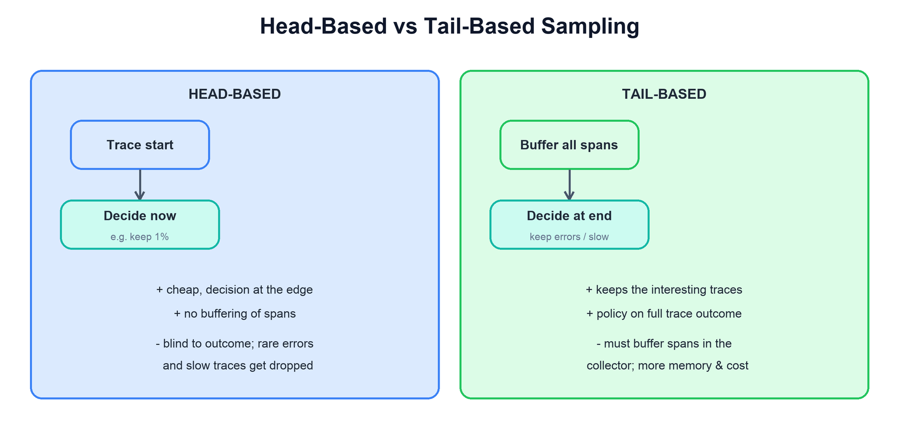
- Head-based sampling. The decision is made when the trace starts, at the edge, and propagated via the sampled flag so all services agree. It is cheap and needs no buffering, but it is blind to the outcome: a 1% head sample keeps 1% of errors too, so most failures and slow requests — exactly what you want — are thrown away.
- Tail-based sampling. The decision is deferred until the whole trace is complete, so the collector can apply policies on the full outcome: keep 100% of traces with an error, keep all traces slower than a threshold, keep a small percentage of normal ones. It captures the interesting traces, but requires buffering all spans of every in-flight trace in the collector (grouped by
trace_id) until it decides — more memory, more complexity, and the collector tier must route all spans of a trace to the same instance.
Real systems (and Grafana Tempo, Jaeger with a tail-sampling collector) often combine them: light head sampling to shed obvious volume cheaply, plus tail sampling to guarantee errors and slow traces are always kept. State this hybrid in an interview — it shows you understand each one’s failure mode.
| Aspect | Head-based | Tail-based |
|---|---|---|
| When | At trace start | After trace completes |
| Buffering | None | All spans, per trace, until decision |
| Keeps errors/slow? | No — blind to outcome | Yes — policy on full trace |
| Cost | Cheap | Memory + routing complexity |
7. Storage, Assembly & Dependency Graphs
Storage. The access pattern is “fetch all spans for a trace_id,” so spans are stored keyed by trace_id. The cost-effective modern design (Grafana Tempo is the clearest example) keeps only a minimal index and writes span blocks to cheap object storage: you do not build a heavy search index over every span attribute; you look up by trace id, and support attribute search via a lighter secondary index or by scanning columnar blocks. This decouples storage cost from compute and is what makes petabyte retention affordable.
Trace assembly. Because spans arrive independently and out of order, the read side collects all spans sharing a trace_id and rebuilds the tree from parent_span_id links, then lays them on a timeline to produce the waterfall. Assembly is a read-time (or collector-time) operation; the write path never needs a complete trace.
Dependency graph & latency analysis. Aggregating across many traces yields a service dependency graph — which service calls which, how often, and with what latency and error rate — and per-operation latency breakdowns that reveal where the critical path spends its time. This aggregate view, computed from sampled traces, is often as valuable as any single trace: it shows the shape of the system and where to look when a whole tier degrades.
Correlation. Because the trace_id and span_id are injected into logs and attached to metric exemplars, a trace is the hub that ties the three observability pillars together — jump from a slow span to its logs, or from a metric spike’s exemplar to the trace.
8. Bottlenecks & Tradeoffs
- Sampling rate vs fidelity. Sample too aggressively and you miss the trace you needed; too little and you cannot afford storage. Tail sampling on errors/latency is the best fidelity-per-byte, at the cost of collector complexity.
- Instrumentation overhead vs coverage. More spans give more detail but add CPU and export volume. Auto-instrument the framework layer; add manual spans only where they earn their keep.
- Tail-sampling routing. Tail sampling requires all spans of a trace to reach the same collector instance, so the collector tier must shard by
trace_id— a real operational constraint that head sampling avoids. - Propagation gaps. A single service that does not propagate context breaks the trace into disconnected fragments. Coverage must be near-universal, which is why a standard (W3C + OpenTelemetry) matters.
- Index cost vs search. A full index over span attributes enables rich search but costs as much as the data; a minimal trace-id index (Tempo-style) is cheap but limits attribute search. Choose based on how users query.
- Clock skew. Spans come from different machines, so unsynchronized clocks distort the waterfall. Rely on causal parent/child ordering and good time sync, not absolute timestamps alone.
9. Summary
A distributed tracing system tags each request with a trace id, propagates it across every hop, and emits timed spans that a backend reassembles into a causal timeline — using sampling to keep the interesting traces affordably.
| Concern | Mechanism |
|---|---|
| What is the data model? | Span = timed unit of work; trace = spans sharing a trace_id, linked by parent_span_id into a tree. |
| How does one request stay one trace? | Context propagation: inject/extract the trace_id at every hop (W3C traceparent, incl. queues). |
| How do we instrument cheaply? | OpenTelemetry SDK: auto-instrument frameworks + manual spans; async export, low overhead. |
| How do we avoid storing everything? | Sampling — head (cheap, blind) + tail (buffers trace, keeps errors/slow); usually hybrid. |
| Where do spans live? | Keyed by trace_id on cheap object storage with a minimal index (Tempo-style). |
| How is a trace rebuilt? | Read-time assembly: gather spans by trace_id, rebuild the tree from parent links, lay on a timeline. |
| What aggregate value is there? | Service dependency graph and latency breakdowns from many traces; correlation to logs/metrics. |