Designing a Capacity Forecasting System
A system design interview guide to predicting when you will run out of hardware — turning utilization telemetry into a demand forecast, a buffer policy, and a procurement order that lands before the wall does.
Fleets do not run out of capacity suddenly; they run out predictably, and the failure is almost always organizational rather than technical — nobody ordered the machines in time. Hardware has a long lead time: you cannot conjure a rack the day you need it, so you must see the shortfall coming weeks or months ahead and place the order early. A capacity forecasting system is the machine that makes that foresight routine. It ingests utilization telemetry, models future demand from trend, seasonality, and known growth, translates that demand into hardware and dollars, applies a headroom policy so you never run to the edge, and alerts — with enough runway — when a resource is projected to exhaust. This guide is infra-economics flavored: the output is not a dashboard, it is a purchase order placed at the right time.
Contents
1. Requirements & Scope
The system’s job is to answer one question reliably: for each resource, when will demand exceed supply, and what should we buy to prevent it? Everything else serves that.
- Ingest. Collect utilization and growth telemetry across resources — compute, memory, storage, network — per service, region, and hardware type.
- Forecast. Project demand forward over the planning horizon, capturing trend, seasonality, and known future events.
- Translate. Convert forecasted demand into hardware units and cost, against a headroom/buffer policy.
- Alert. Warn when a resource is projected to breach its buffer, with enough lead time to procure before exhaustion.
- What-if. Let planners model scenarios — a launch, a migration, a region build-out — and see the capacity impact.
- Non-goals. Real-time autoscaling (minutes-scale reaction) is a different system; forecasting operates on the weeks-to-quarters horizon where procurement lives.
2. Back-of-the-Envelope
The numbers here are about horizons and lead times, because those set how far ahead the forecast must see and how early the alert must fire.
| Quantity | Assumption | Result |
|---|---|---|
| Telemetry cadence | utilization sampled every 1–5 min | plenty of history; downsample to hourly/daily for modeling |
| Series count | resource × service × region × HW type | tens of thousands of forecastable series |
| Planning horizon | forecast 2–4 quarters ahead | needs 1–2 years of history to learn seasonality |
| Procurement lead time | order → racked & serving | weeks to months — the number that matters most |
| Headroom buffer | N+2 / keep ~20–30% free | absorb spikes + one failure domain |
| Alert runway | fire before exhaustion by | ≥ lead time + safety margin |
The controlling number is procurement lead time. It defines the alert runway: if hardware takes eight weeks to arrive, a projected-exhaustion alert that fires four weeks out is useless. The whole system exists to convert a slow physical process (buying and racking machines) into a timely one by seeing far enough ahead.
3. Key Definitions
A shared vocabulary keeps the design honest, especially around what “capacity” and “headroom” actually mean.
| Term | Meaning |
|---|---|
| Demand | Forecasted resource need over time — what the workload will consume. |
| Supply / capacity | Provisioned resource available — what the fleet can serve. |
| Headroom | Free capacity above current demand — the safety margin. |
| Buffer policy | The rule for how much headroom to keep (e.g. N+2, or 25% free). |
| Days-to-exhaustion | Time until forecasted demand crosses the usable-capacity line. |
| Lead time | Delay from ordering hardware to it serving traffic. |
| Order point | The moment you must order so hardware lands before the buffer is breached. |
The core relationship: order point = exhaustion date − lead time − safety margin. The forecast’s only real purpose is to compute that date early enough to act on it.
4. High-Level Architecture
The system is a pipeline from raw telemetry to a procurement decision, with a planning loop hanging off the middle for what-if analysis.
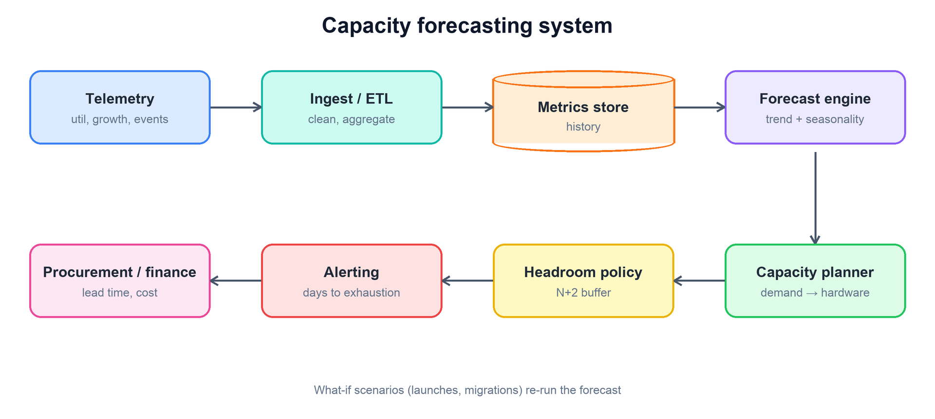
- Telemetry. Utilization, growth, and event signals collected across the fleet, tagged by resource, service, region, and hardware type.
- Ingest / ETL. Cleans, normalizes, and downsamples raw samples into the coarser resolution modeling needs, handling gaps and outliers.
- Metrics store. A time-series store holding the long history — a year or two — that the models learn from.
- Forecast engine. Fits per-series models and projects demand forward with uncertainty bands.
- Capacity planner. Converts forecasted demand into hardware units and cost, and compares against supply plus the headroom policy.
- Alerting & integration. Fires projected-exhaustion alerts with runway, and feeds the plan to procurement and finance.
5. Modeling Demand
Forecasting demand starts by recognizing that a utilization time series is not random — it is a few structured components plus noise. Decompose it, model each part, and recombine.
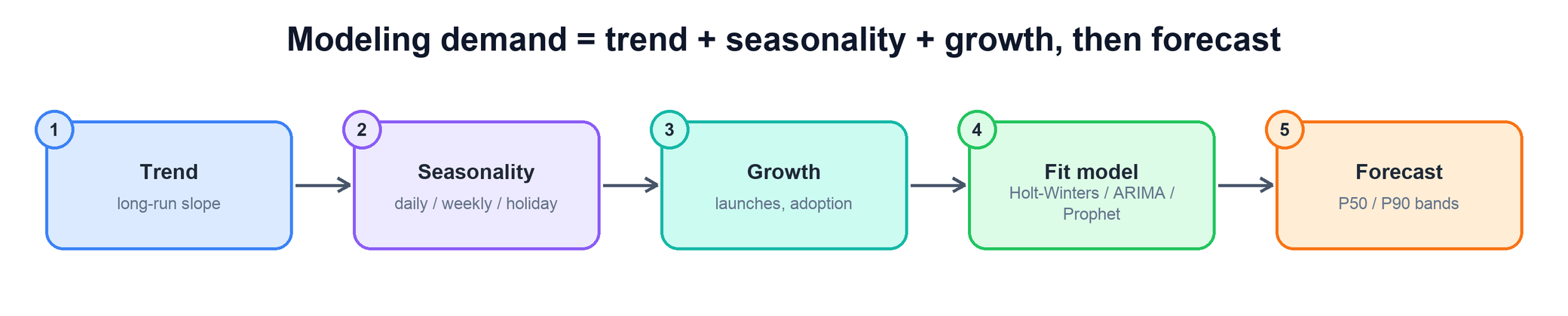
- Trend. The long-run slope — steady organic growth or decline.
- Seasonality. Repeating cycles: daily peaks, weekly patterns, holiday and end-of-quarter surges. Missing these makes a forecast dangerously optimistic at exactly the wrong time.
- Growth events. Known step changes — a product launch, a new region, a migration — that history alone cannot predict and must be injected as regressors.
- Residual / noise. What is left after the structured parts — the irreducible uncertainty that sets the width of the confidence band.
Classic model choices: Holt-Winters (exponential smoothing with trend and seasonality) is simple and robust; ARIMA / SARIMA handles autocorrelation and seasonality with more rigor; Prophet is convenient for series with strong seasonality and holiday effects and tolerates gaps. The key output is not a single line but a distribution: forecast at P50 for the expected case and at P90 for planning, because you provision against a pessimistic percentile, not the average. You buy for the bad month, not the typical one.
for series in resources:
  hist   = store.history(series, window="2y")
  parts  = decompose(hist)                # trend + seasonality + residual
  model  = fit(parts, extra=known_events) # inject launches/migrations
  fc     = model.forecast(horizon,
                          quantiles=[0.5, 0.9]) # plan against P90
  publish(series, fc)
6. Headroom & Exhaustion
A forecast of demand only becomes actionable when compared to supply through a headroom policy. You never plan to fill capacity to 100% — you keep a buffer for spikes, for a failed failure-domain, and for the forecast’s own error.
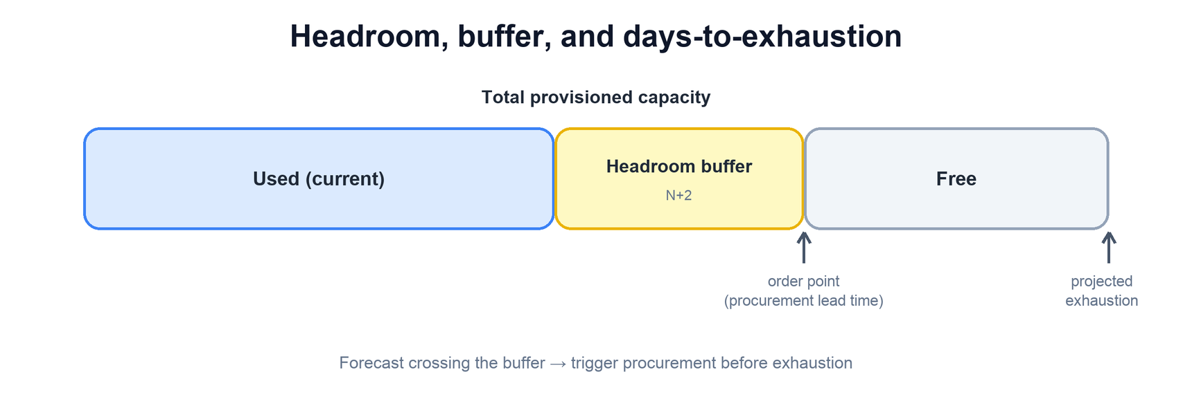
The buffer policy encodes the safety margin: N+1 or N+2 (survive one or two failure domains going down at peak), or a simple “keep 25% free.” Usable capacity is provisioned capacity minus the buffer, and the alert fires when the forecast — not current usage — is projected to cross that usable line within the lead-time runway. Alerting on the projection rather than the present is the whole point: by the time current usage hits the wall, it is far too late to order.
usable          = capacity - buffer(policy)          # e.g. N+2 or 25% free
exhaustion_date = first_day(forecast.p90 > usable)   # pessimistic percentile
order_point     = exhaustion_date - lead_time - margin
if today >= order_point:
  alert("procure now", resource, exhaustion_date, units_needed) # runway preserved
7. What-If & Procurement
The forecast is a baseline; the value multiplies when planners can perturb it and when its output flows straight into the buying process.
- What-if scenarios. A planner overlays a hypothetical — “this launch adds 30% load in Q3,” “we migrate service X to a new region,” “we retire this hardware generation” — and the engine re-runs the forecast to show the capacity and cost impact. This turns forecasting from a passive report into a planning tool.
- Cost translation. Demand is expressed not just in cores and terabytes but in dollars, using per-unit hardware and running costs, so capacity decisions can be weighed as budget decisions. Infra planning is fundamentally an economics exercise.
- Procurement & finance integration. The plan feeds the systems that actually order hardware and hold the budget. An order-point alert becomes a procurement request; the aggregated forecast becomes the quarterly capex ask. The loop closes only when the forecast changes what gets bought.
8. Bottlenecks & Tradeoffs
Forecasting trades the cost of being wrong in one direction against the cost of being wrong in the other, and the design is mostly about choosing which error to prefer.
- Over- vs under-provisioning. Provision too much and you burn budget on idle hardware; too little and you hit a wall and take an outage or throttle growth. A bigger buffer and higher percentile favor safety at a cost; the right balance depends on how expensive an outage is versus idle capacity.
- Model accuracy vs simplicity. A fancier model may fit better but is harder to trust, explain, and maintain. Simple, robust models (Holt-Winters) that planners understand often beat opaque ones, especially when the output drives real spend.
- Horizon vs uncertainty. Forecasts degrade the further out you look, yet lead time forces a long horizon. You manage this by widening bands with distance and re-forecasting continuously as new data arrives, rather than committing once.
- Seasonality traps. A model blind to a holiday or quarter-end surge under-forecasts exactly when demand peaks. Capturing seasonality — and injecting known one-off events — is where forecasts most often fail in practice.
- Data quality. Garbage telemetry yields garbage forecasts. Gaps, outliers from incidents, and metric changes must be cleaned or the model learns the wrong shape — an outage’s dip should not be read as falling demand.
9. Summary
A capacity forecasting system converts slow physical procurement into timely action by seeing demand far enough ahead. Its deliverable is a well-timed order, and every part of the design serves the order point.
| Concern | Mechanism |
|---|---|
| What do we feed the model? | Cleaned, downsampled utilization/growth telemetry with 1–2 years of history. |
| How do we model demand? | Decompose into trend + seasonality + growth; fit Holt-Winters / ARIMA / Prophet. |
| What do we forecast against? | A pessimistic percentile (P90) with uncertainty bands — provision for the bad case. |
| How much slack do we keep? | A headroom buffer (N+2 or ~25% free) subtracted from provisioned capacity. |
| When do we alert? | When the forecast (not current usage) is projected to breach the buffer within the runway. |
| How early must the alert be? | At least procurement lead time plus a safety margin — the order point. |
| How do we plan changes? | What-if scenarios re-run the forecast; output translates to hardware and cost. |
| How does it drive action? | Integration with procurement and finance turns alerts into orders and capex plans. |