Apache Cassandra — Internal Architecture
A developer's guide to how Cassandra actually works under the hood: cluster architecture, the storage engine, replication, the Log-Structured Merge tree, and how data moves when nodes join or leave.
Apache Cassandra is a distributed, wide-column NoSQL database designed for high write throughput, linear horizontal scalability, and no single point of failure. Its design borrows two big ideas: the data distribution and replication model from Amazon Dynamo (consistent hashing, tunable consistency, gossip, hinted handoff) and the on-disk storage model from Google Bigtable (the Log-Structured Merge tree, memtables, and SSTables). Understanding Cassandra means understanding how those two halves fit together.
Contents
1. Design Goals and Core Ideas
Every internal decision in Cassandra traces back to a small set of goals. Keeping them in mind makes the rest of the architecture predictable.
| Goal | How Cassandra achieves it |
|---|---|
| No single point of failure | Fully peer-to-peer. Every node is identical; there is no master, no name node, no config server. |
| Linear scalability | Data is partitioned across nodes by a hash ring. Adding nodes adds capacity proportionally. |
| High write throughput | Writes are append-only (commit log + in-memory memtable). No read-before-write, no in-place updates. |
| Tunable consistency | The client chooses, per query, how many replicas must respond. Trade latency against consistency. |
| Always-on availability | An AP system (in CAP terms). It favors availability and partition tolerance; consistency is tunable, not absolute. |
2. Cluster Architecture
A Cassandra cluster is a ring of identical, equal peers. There is no coordinator process and no leader election for data ownership. Any node can accept any request; the node that receives a client request becomes the coordinator for that single request and routes it to the nodes that own the data.
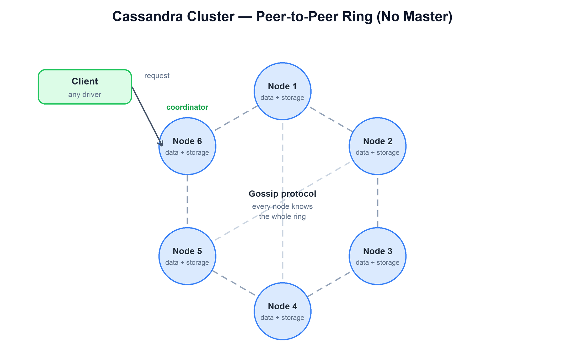
The key components running on every node are:
- Coordinator role: a transient, per-request role. The coordinator forwards reads and writes to the correct replicas, gathers responses, and applies the consistency level before replying to the client.
- Gossip: a peer-to-peer protocol that runs once per second. Each node exchanges state (which nodes are up, their tokens, their schema version, their load) with a few random peers. Within a few rounds, state propagates to the whole cluster. No node needs a central registry.
- Snitch: the component that tells Cassandra the network topology — which rack and which datacenter each node lives in. The replica-placement strategy uses this to spread replicas across failure domains.
- Partitioner: the hash function (Murmur3Partitioner by default) that maps a partition key to a token, deciding which node owns the row.
3. Data Distribution: Partitioning and the Token Ring
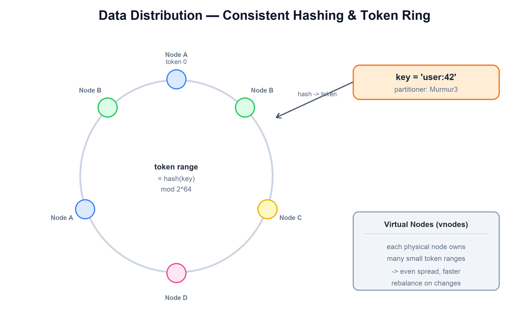
Cassandra distributes data using consistent hashing. The entire output space of the hash function (a 64-bit signed integer for Murmur3) is treated as a ring. Each node is assigned one or more tokens — positions on the ring. A node owns the range of tokens from the previous node's token (exclusive) up to its own token (inclusive).
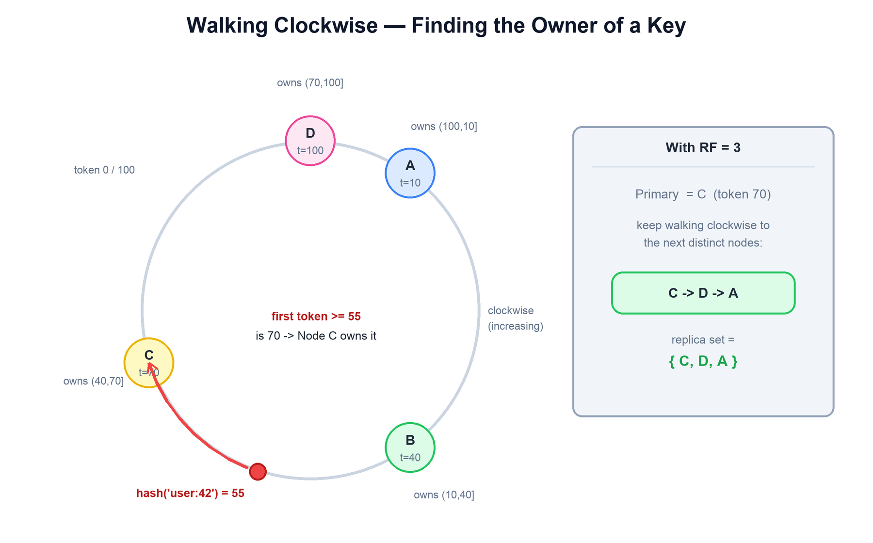
To locate a row, Cassandra hashes its partition key to a token, then walks clockwise around the ring to find the first node whose range contains that token. That node is the first replica; the next N-1 nodes clockwise hold the additional copies.
A concrete walk-clockwise example
Picture the ring as the numbers 0 to 100 wrapping back to 0, with four single-token nodes: A at token 10, B at 40, C at 70, and D at 100. Each node owns the range from its predecessor's token (exclusive) up to its own token (inclusive), so A owns (100,10], B owns (10,40], C owns (40,70], and D owns (70,100]. If hash('user:42') resolves to 55, you start at 55 and move in the direction of increasing tokens; the first token you reach is 70, so Node C owns the row. For RF=3 you keep walking clockwise to the next distinct physical nodes, which gives the replica set { C, D, A }.
Virtual nodes (vnodes): naming and mapping
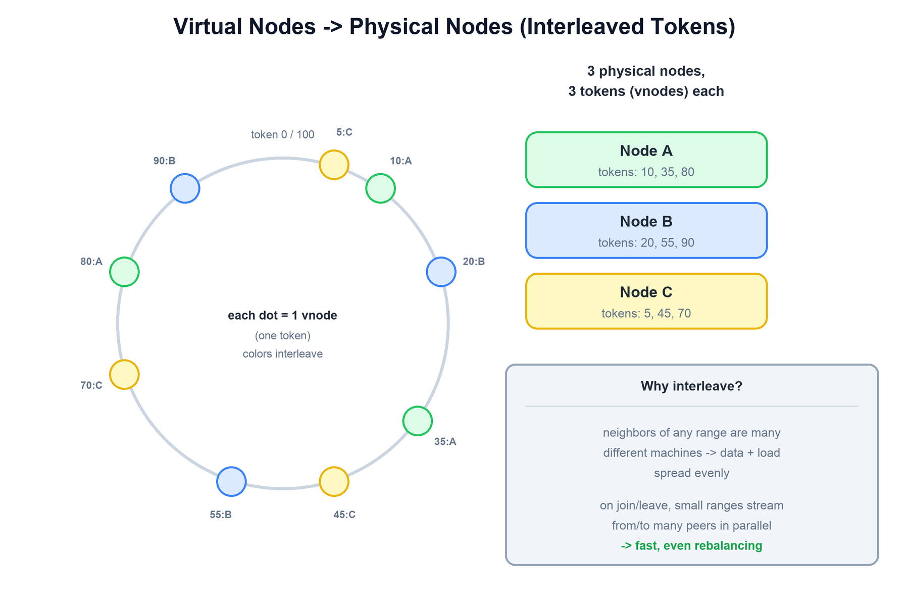
Instead of one large token range per machine, each physical node is assigned many small ranges scattered around the ring (16 in modern Cassandra, 256 historically). This spreads data and load more evenly and, critically, makes rebalancing faster — when a node joins or leaves, many small ranges are streamed from many peers in parallel rather than one huge range from a single neighbor.
A virtual node is not a named process — it is simply one token, identified by its token value (a 64-bit integer for Murmur3). Each physical node is configured with num_tokens and on join is assigned that many tokens. Each assigned token defines one vnode range, so "owning 16 vnodes" means owning the 16 ranges whose upper-bound tokens belong to that node. The cluster maintains a single sorted token-to-endpoint map — each physical node has a host-ID (a UUID) and an address — and gossip distributes this map so any node can resolve any token to its owning machine. The mapping is many-to-one and interleaved: consecutive tokens on the ring usually belong to different physical nodes, which is exactly what spreads data evenly and lets bootstrap and decommission stream from many peers in parallel.
The routing logic on the coordinator is straightforward:
function route(partition_key):
  token = murmur3(partition_key)        # 64-bit signed int
  primary = ring.find_owner_clockwise(token)
  replicas = []
  node = primary
  while len(replicas) < replication_factor:
    if placement_strategy.accepts(node, replicas):   # rack/DC aware
      replicas.append(node)
    node = ring.next_clockwise(node)
  return replicas
4. Replication
The replication factor (RF) defines how many copies of each row exist. With RF=3, every row is stored on three nodes. Replica placement is governed by a strategy:
- SimpleStrategy: places replicas on the next N-1 nodes clockwise. Topology-unaware; for a single datacenter only.
- NetworkTopologyStrategy: places replicas to satisfy a per-datacenter RF, walking the ring while skipping nodes until it has spread copies across distinct racks. This is the production choice.
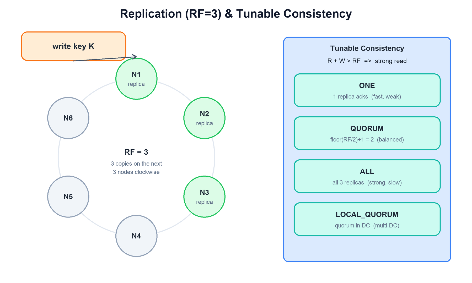
Tunable consistency is the second half of the Dynamo model. Each query specifies a consistency level (CL) — how many replicas must acknowledge before the operation is considered successful. The fundamental rule is that if R + W > RF (read replicas plus write replicas exceed the replication factor), every read is guaranteed to see the latest acknowledged write, because the read and write quorums always overlap on at least one node.
Cassandra keeps replicas consistent over time through three anti-entropy mechanisms:
| Mechanism | When it runs | What it does |
|---|---|---|
| Read repair | During a read | If replicas return different values, the coordinator pushes the newest version back to the stale replicas. |
| Hinted handoff | During a write, when a replica is down | The coordinator stores a "hint" and replays the write to the replica once it comes back online. |
| Repair (Merkle trees) | Scheduled / manual (nodetool repair) | Replicas compare Merkle-tree hashes of their data and stream only the differing ranges to reconcile. |
The coordinator's write logic under a consistency level:
function write(key, value, CL):
  replicas = route(key)
  required = consistency_count(CL, replication_factor)   # QUORUM -> floor(RF/2)+1
  acks = 0
  for r in replicas:
    if r.is_alive():
      send_async(r, key, value)     # r appends to commit log + memtable
    else:
      store_hint(r, key, value)     # hinted handoff
  wait until acks >= required        # count only successful replica responses
  return SUCCESS                     # remaining replicas keep applying in the background
5. The Storage Engine: Log-Structured Merge Tree
Cassandra's on-disk engine is a Log-Structured Merge tree (LSM). The central idea: never modify data in place. All writes are sequential appends, which is far faster than random disk I/O. Updates and deletes become new entries; the system reconciles versions at read time and during background compaction.
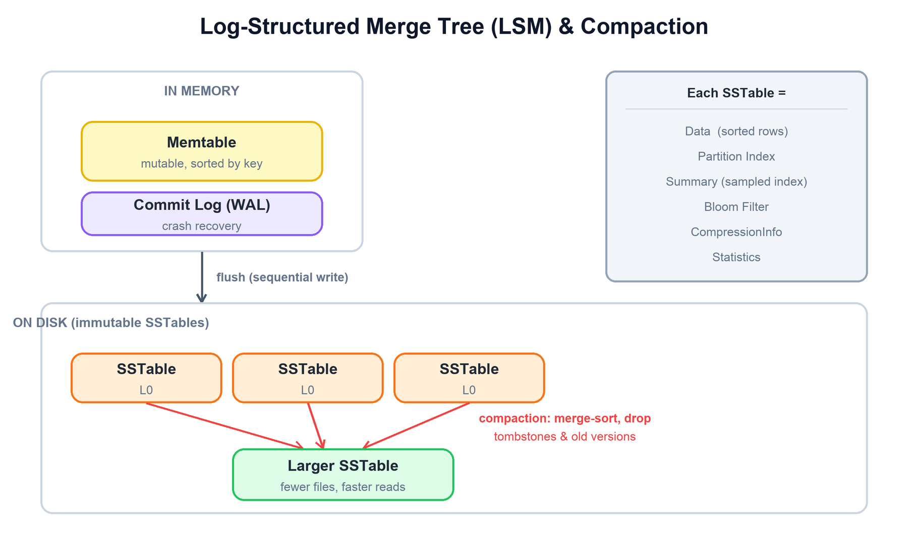
The three core structures are:
- Commit log: an append-only write-ahead log on disk. Its only job is durability — if a node crashes before a memtable is flushed, the commit log is replayed on restart to recover.
- Memtable: an in-memory, sorted structure (per table) that holds recent writes. It is fast and mutable. When it reaches a threshold, it is flushed.
- SSTable (Sorted String Table): an immutable, sorted file on disk produced by flushing a memtable. Because it is immutable, it never needs locking and can be read concurrently. Each SSTable ships with auxiliary structures: a bloom filter (to skip files that cannot contain a key), a partition index and a sampled summary (to seek directly to a key), plus compression and statistics metadata.
Compaction is the background process that merges multiple SSTables into fewer, larger ones. It performs a merge-sort, keeps only the newest version of each cell, and physically removes tombstones (deletion markers) once they are older than gc_grace_seconds. Compaction is what keeps read amplification under control. The main strategies are:
| Strategy | Best for |
|---|---|
| STCS (Size-Tiered) | Write-heavy workloads. Merges SSTables of similar size. Default. |
| LCS (Leveled) | Read-heavy workloads. Keeps small, non-overlapping levels for predictable read latency. |
| TWCS (Time-Window) | Time-series data with TTLs. Groups data by time window for cheap expiry. |
6. Write Path
A write is acknowledged the moment it is durable in the commit log and visible in the memtable. There is no read-before-write and no random disk seek on the hot path, which is why Cassandra writes are so fast.
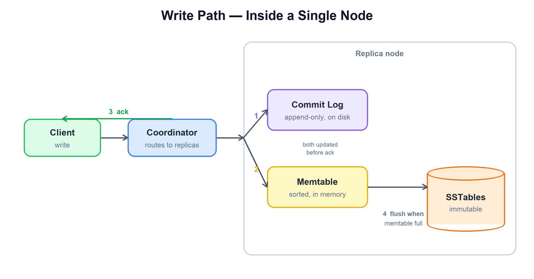
Inside a replica, a single write proceeds as:
function apply_write(key, value):
commit_log.append(key, value) # 1. durability (sequential disk write)
memtable.put(key, value) # 2. in-memory, sorted
ack() # 3. respond to coordinator
if memtable.size() > threshold: # 4. flush, asynchronously
sstable = memtable.flush_to_disk() # immutable, sorted
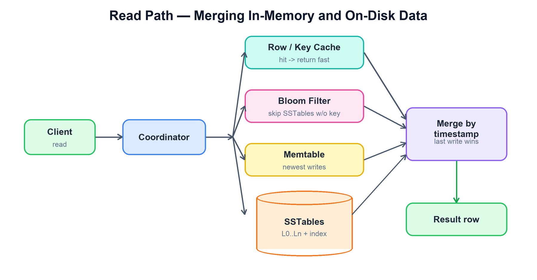
commit_log.discard(segments_covered_by(sstable))7. Read Path
A read is more involved than a write because the current value of a row may be spread across the memtable and several SSTables (each holding a different version or column). The coordinator gathers candidate data from all sources and merges by timestamp — last write wins at the cell level.
On a single replica, the local read works like this:
function read(key):
  if row_cache.contains(key): return row_cache.get(key)   # fast path
  candidates = []
  candidates += memtable.get(key)   # newest, in memory
  for sstable in sstables:
    if not sstable.bloom_filter.might_contain(key):
      continue                      # skip files that cannot hold the key
    offset = sstable.index.lookup(key)     # partition index / summary
    candidates += sstable.read_at(offset)
  row = merge_by_timestamp(candidates)     # last write wins; drop tombstoned cells
  row_cache.put(key, row)
  return row
The bloom filter is the key optimization: it lets a replica skip SSTables that definitely do not contain the requested key, avoiding pointless disk reads. A delete does not erase data; it writes a tombstone that shadows older versions until compaction physically removes them.
8. Membership and Failure Detection
Because there is no master, nodes must agree on who is alive entirely through gossip. Once per second, each node picks a few random peers and exchanges a digest of everything it knows about every node — heartbeat counters and application state. Newer information (higher version numbers) overwrites older information, so the cluster state converges quickly.
Failure detection is not a simple timeout. Cassandra uses a Phi Accrual Failure Detector, which outputs a continuous suspicion level (phi) based on the statistical distribution of recent heartbeat inter-arrival times, rather than a binary up/down. A node is marked down only when phi crosses a configured threshold, which adapts to real network conditions and reduces false positives.
every 1 second on each node:
  my_heartbeat += 1
  peers = pick_random_live_peers(count=3)
  for p in peers:
    send(p, my_view_of_cluster)     # digests + states
  # on receiving a peer's view, merge: keep entries with the higher version

function is_down(node):
  phi = -log10(P(now - last_heartbeat[node]))   # accrual
  return phi > PHI_THRESHOLD          # e.g. 8
9. Adding a Node (Scaling Out)
Adding a node is called bootstrapping. The new node is assigned tokens (with vnodes, many small ranges spread around the ring). It now becomes a replica for those ranges, so it must receive the corresponding data from the nodes that currently hold it before it can serve reads.
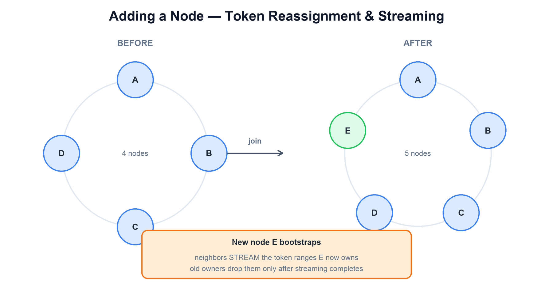
The bootstrap sequence is:
- The new node starts, contacts a seed node, and learns the ring topology through gossip.
- It calculates the token ranges it will own and announces a JOINING state.
- Neighbors that currently own those ranges stream the relevant SSTable data to the new node, in parallel across many vnode ranges.
- Once streaming completes, the node transitions to NORMAL and begins serving reads and writes for its ranges.
- The previous owners now hold redundant copies. An operator runs
nodetool cleanupon them to delete data they no longer own and reclaim disk.
on new_node bootstrap:
  contact_seed(); learn_ring_via_gossip()
  my_ranges = compute_owned_ranges(my_tokens)
  announce(state = JOINING)
  for range in my_ranges:
    source = current_owner(range)
    stream_sstables_from(source, range)   # parallel
  announce(state = NORMAL)                 # now serves traffic
# operator later: nodetool cleanup on old owners
10. Removing a Node (Scaling In or Replacing Failure)
Removing a node must preserve the replication factor: every range the departing node held must still have RF copies afterward. The procedure depends on whether the node is alive.
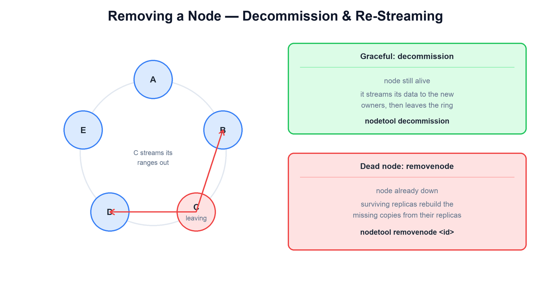
| Scenario | Command | What happens |
|---|---|---|
| Node is alive (graceful scale-in) | nodetool decommission | The leaving node itself streams each of its ranges to the new owners (the next replica clockwise), then leaves the ring. RF is preserved throughout. |
| Node is dead (hardware failure) | nodetool removenode <id> | The dead node cannot stream anything. The surviving replicas that still hold copies of its ranges rebuild the now-missing third copy by streaming among themselves. |
| Replace in place | replace_address flag | A fresh node takes over the dead node's exact tokens and bootstraps the data from the remaining replicas. |
In all cases the ring re-forms automatically through gossip, and the affected token ranges end up with the full replication factor of copies again. No central coordinator orchestrates this; it is driven by the nodes that own the affected ranges.
decommission (node alive):
  announce(state = LEAVING)
  for range in my_ranges:
    new_owner = next_replica_clockwise(range)
    stream_sstables_to(new_owner, range)
  announce(state = LEFT); shut_down()

removenode (node dead):
  for range owned by dead_node:
    survivors = live_replicas(range)
    new_owner = next_replica_clockwise(range)
    stream_sstables(from = survivors, to = new_owner)
11. Summary
The whole system is built from a few reinforcing ideas:
| Concern | Mechanism |
|---|---|
| Where does a row live? | Consistent hashing of the partition key onto a token ring; vnodes for even spread. |
| How many copies? | Replication factor, placed by a topology-aware strategy. |
| How consistent? | Tunable consistency level per query; R + W > RF gives strong reads. |
| How are writes so fast? | Append-only commit log + in-memory memtable; no in-place updates. |
| How is data stored and reclaimed? | Immutable SSTables (LSM), reconciled and compacted in the background. |
| How do nodes coordinate? | Gossip + Phi Accrual failure detection; no master. |
| How does it scale? | Bootstrap streams ranges in; decommission/removenode streams them out. RF is preserved throughout. |