Basic Algorithms & Patterns
A quick-reference deck of the core algorithmic patterns behind most coding problems — recognize the pattern, then reach for the right algorithm. Minimal words: the pseudocode is the reference and one diagram per algorithm shows the mechanic.
Most interview and day-to-day algorithm problems are variations on a small set of reusable patterns. Learn to recognize the pattern from the shape of the problem — sorted input, a contiguous range, a graph, overlapping subproblems — and the algorithm usually follows. This page groups the essential algorithms under the pattern each one exemplifies: each pattern gets a short intro on when it applies, then its algorithms as compact pseudocode with a schematic diagram.
Contents
1. Two Pointers
Use two indices that walk a sequence — usually from opposite ends, sometimes at different speeds — to replace a nested-loop scan with a single linear pass. The core idea is that each step provably discards one candidate, so the whole sweep is O(n) time and O(1) space. Works best on sorted or symmetric data.
Pair sum in a sorted array
Start one pointer at each end and move them inward based on how the current sum compares to the target. Because the array is sorted, every move eliminates exactly one impossible partner.
function pair_sum(arr, target):    # arr is sorted ascending
  lo = 0
  hi = length(arr) - 1
  while lo < hi:
    sum = arr[lo] + arr[hi]
    if sum == target: return (lo, hi)  # found it
    if sum < target: lo = lo + 1       # need a bigger value
    else:            hi = hi - 1        # need a smaller value
  return NONE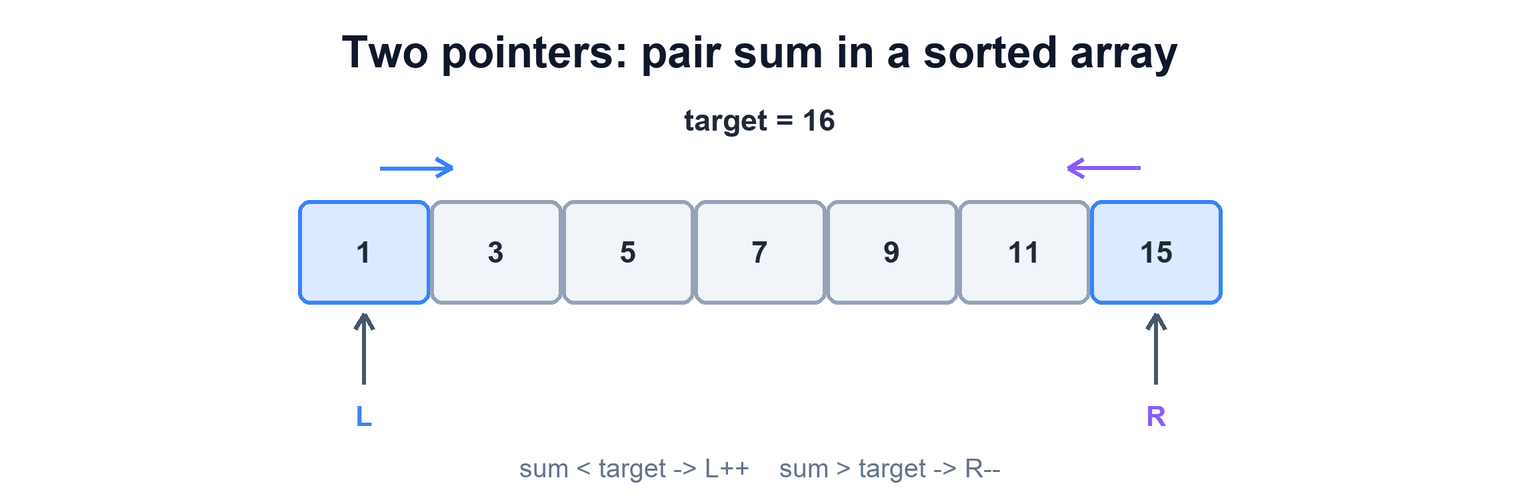
Reverse / palindrome check
Swap the outermost pair, then step both pointers inward; the same walk either reverses in place or verifies a palindrome by comparing instead of swapping.
function reverse(arr):
  lo = 0
  hi = length(arr) - 1
  while lo < hi:
    swap(arr[lo], arr[hi])   # or: compare for palindrome
    lo = lo + 1
    hi = hi - 1
  return arr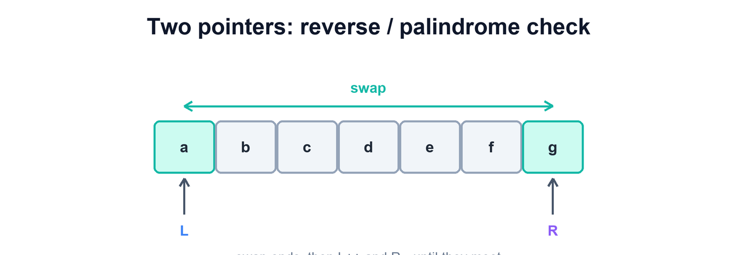
2. Sliding Window
Use a moving window over a contiguous run of a sequence to answer questions about subarrays or substrings without recomputing from scratch. The core idea is to add the entering element and remove the leaving element as the window moves, keeping each step O(1) for an overall O(n) pass. The window is either a fixed size or grows and shrinks on a condition.
Max-sum subarray of size k (fixed window)
Keep a running sum of exactly k elements; on each slide subtract the element that leaves and add the one that enters, so the sum updates in constant time.
function max_sum_k(arr, k):
  window = sum(arr[0 .. k-1])   # first window
  best = window
  for right in k .. length(arr)-1:
    window = window + arr[right] - arr[right - k]  # add new, drop old
    best = max(best, window)
  return best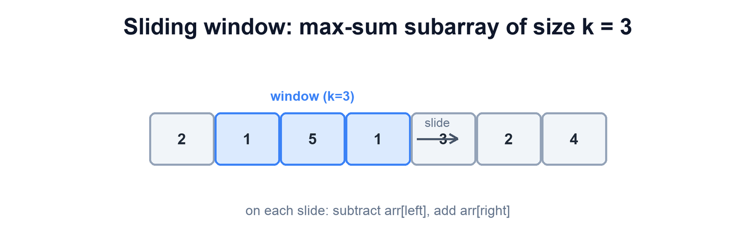
Longest substring without repeating characters (variable window)
Grow the window by advancing the right edge; when a duplicate appears, shrink from the left until the window is valid again, tracking the best length seen.
function longest_unique(s):
  seen = empty set
  left = 0
  best = 0
  for right in 0 .. length(s)-1:
    while s[right] in seen:        # duplicate -> shrink
      remove s[left] from seen
      left = left + 1
    add s[right] to seen           # extend window
    best = max(best, right - left + 1)
  return best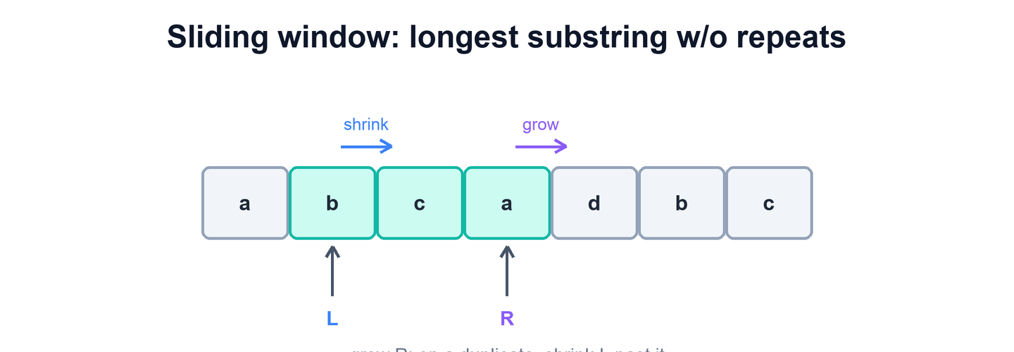
3. Fast & Slow Pointers
Use two pointers advancing at different speeds over a linked structure to detect cycles or find a midpoint without extra memory. The core idea is that if a loop exists the fast pointer laps the slow one and they collide; otherwise fast simply runs off the end. Time is O(n) with O(1) space.
Linked-list cycle detection (Floyd’s)
Advance slow by one node and fast by two; if they ever meet the list has a cycle, and if fast reaches the end it does not.
function has_cycle(head):
  slow = head
  fast = head
  while fast != NULL and fast.next != NULL:
    slow = slow.next          # +1 step
    fast = fast.next.next     # +2 steps
    if slow == fast:          # pointers collided
      return TRUE
  return FALSE                # fast ran off the end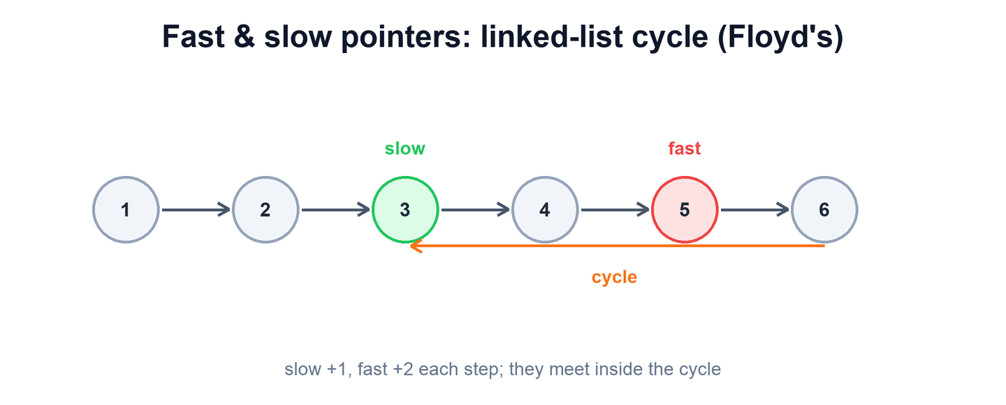
4. Binary Search
Use repeated halving to locate a value in a sorted range, discarding half the candidates at every comparison. The core idea is that an ordered invariant lets you rule out an entire side by looking at one midpoint, giving O(log n) time. It generalizes to any monotonic predicate, not just literal arrays.
Classic binary search
Track a lo/hi range, probe the midpoint, and collapse toward the half that can still contain the target.
function binary_search(arr, target):   # arr sorted ascending
  lo = 0
  hi = length(arr) - 1
  while lo <= hi:
    mid = lo + (hi - lo) / 2   # avoids overflow
    if arr[mid] == target: return mid
    if target < arr[mid]: hi = mid - 1  # search left half
    else:                lo = mid + 1   # search right half
  return NOT_FOUND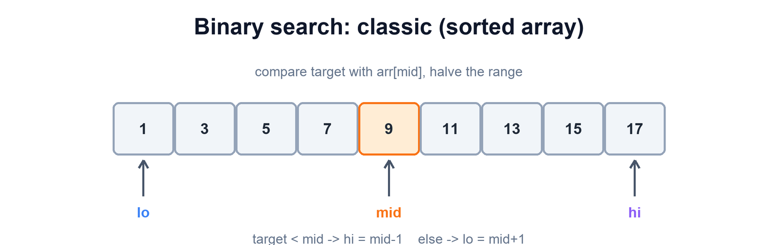
Search in a rotated sorted array
A rotation leaves one half still sorted at every step; decide which half is ordered, and search there only if the target falls inside its range.
function search_rotated(arr, target):
  lo = 0
  hi = length(arr) - 1
  while lo <= hi:
    mid = lo + (hi - lo) / 2
    if arr[mid] == target: return mid
    if arr[lo] <= arr[mid]:               # left half is sorted
      if arr[lo] <= target < arr[mid]: hi = mid - 1
      else:                           lo = mid + 1
    else:                                 # right half is sorted
      if arr[mid] < target <= arr[hi]: lo = mid + 1
      else:                           hi = mid - 1
  return NOT_FOUND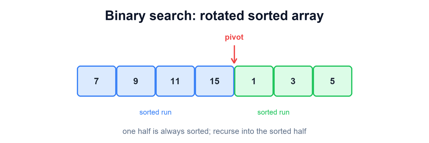
5. Depth-First Search (DFS)
Use DFS to explore a tree or graph by going as deep as possible along each branch before backtracking, via recursion or an explicit stack. The core idea is to fully finish one subtree or region before moving to the next, visiting every node and edge once in O(V + E). It is the natural fit for traversal order, connectivity, and path enumeration.
Tree traversal (pre / in / post-order)
Recurse into the left and right children; the position of the visit relative to those two recursive calls chooses pre-, in-, or post-order.
function dfs(node):
  if node == NULL: return
  visit(node)        # PRE-order: before children
  dfs(node.left)
  # visit(node)      # IN-order: between children
  dfs(node.right)
  # visit(node)      # POST-order: after children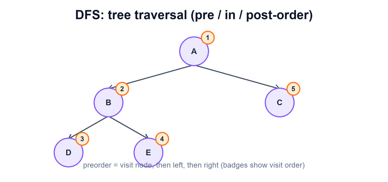
Flood fill / connected components
From a starting cell, recurse into each same-valued neighbor, marking cells visited so the search fills one connected region without revisiting.
function flood(grid, r, c, target, seen):
  if (r, c) out of bounds: return
  if (r, c) in seen or grid[r][c] != target: return
  add (r, c) to seen              # mark visited
  for (dr, dc) in [(-1,0),(1,0),(0,-1),(0,1)]:
    flood(grid, r + dr, c + dc, target, seen)  # 4 neighbors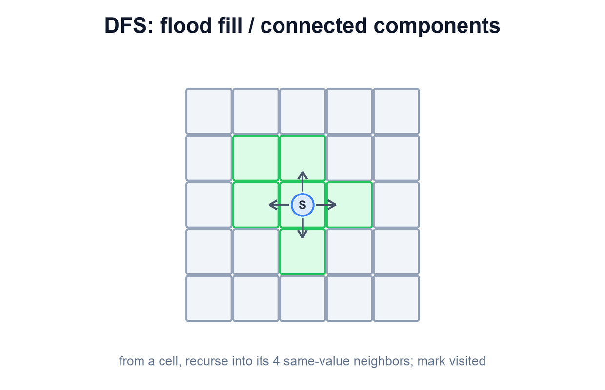
6. Breadth-First Search (BFS)
Use BFS to explore a graph in expanding rings, visiting all nodes at distance k before any at distance k+1, driven by a queue. The core idea is that this level-order sweep reaches every node by its fewest edges, so the first time a node is seen is its shortest hop count. It runs in O(V + E).
Shortest path in an unweighted graph
Seed a queue with the source, then repeatedly dequeue a node and enqueue its unseen neighbors; distances fill in layer by layer.
function bfs(source):
  queue = [source]
  dist = { source: 0 }         # seen + hop count
  while queue not empty:
    node = dequeue(queue)
    for nbr in neighbors(node):
      if nbr not in dist:      # first sighting = shortest
        dist[nbr] = dist[node] + 1
        enqueue(queue, nbr)
  return dist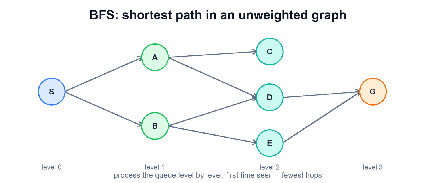
7. Backtracking
Use backtracking to build candidate solutions one choice at a time, abandoning a branch the moment it cannot lead to a valid answer. The core idea is a depth-first walk of the decision tree that undoes each choice on the way back up, pruning dead branches early. Worst case is exponential, but pruning makes many problems tractable.
Subsets / permutations
At each element decide to include it or not, recurse, then undo the choice; the leaves of that binary decision tree enumerate every combination.
function subsets(items, index, current, results):
  if index == length(items):
    results.append(copy(current))   # a complete subset
    return
  subsets(items, index + 1, current, results)   # exclude item
  current.append(items[index])                  # choose
  subsets(items, index + 1, current, results)   # include item
  current.pop()                                 # undo (backtrack)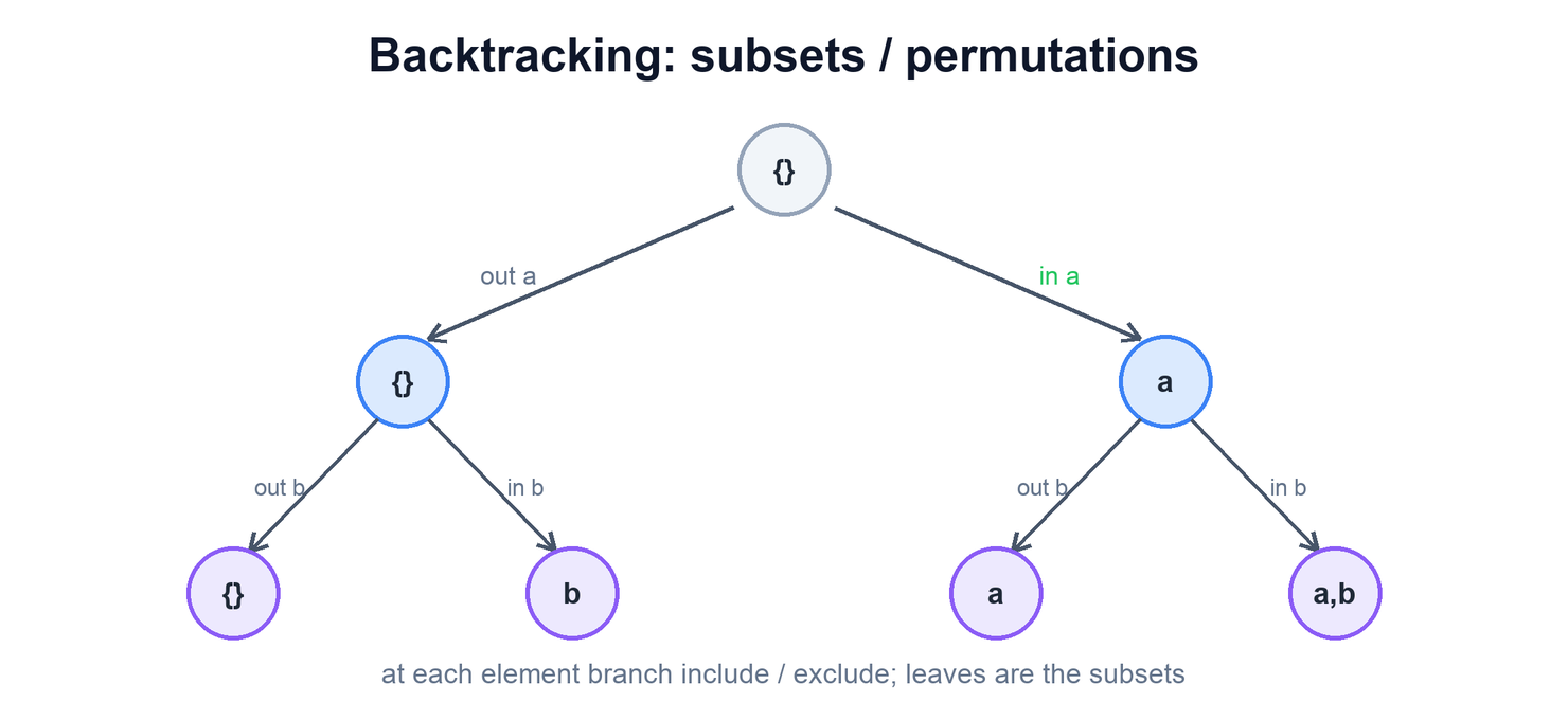
N-Queens
Place one queen per row, trying each column; recurse to the next row only from safe squares and backtrack when a placement is attacked.
function solve(row, n, board):
  if row == n:
    record(board)              # all queens placed
    return
  for col in 0 .. n-1:
    if is_safe(board, row, col):   # no column/diagonal attack
      place queen at (row, col)
      solve(row + 1, n, board)
      remove queen at (row, col)   # backtrack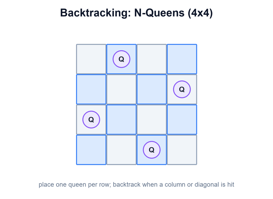
8. Dynamic Programming
Dynamic programming solves a problem by breaking it into overlapping subproblems, solving each once, and reusing the answer — either top-down with a memo or bottom-up with a table.
Fibonacci (memoization vs tabulation)
The naive recursion recomputes the same subproblems exponentially; caching each result (memoization) or filling an array bottom-up (tabulation) makes it linear.
# top-down: memoize the recursion
function fib_memo(n, memo):
  if n ≤ 1: return n
  if n in memo: return memo[n]           # reuse cached subproblem
  memo[n] = fib_memo(n-1, memo) + fib_memo(n-2, memo)
  return memo[n]

# bottom-up: fill a table
function fib_tab(n):
  dp = [0, 1]
  for i from 2 to n:
    dp[i] = dp[i-1] + dp[i-2]            # O(n) time, O(1) space if rolled
  return dp[n]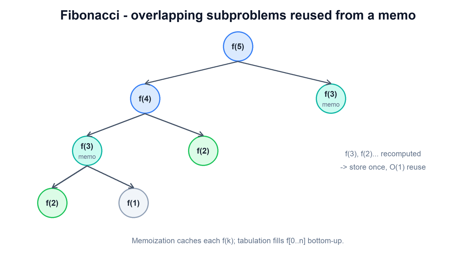
0/1 Knapsack
Choose a subset of items to maximize value within a weight capacity; each cell of the DP grid is the best value for the first i items at capacity w.
function knapsack(weights, values, capacity):
  n = len(weights)
  dp = grid[n+1][capacity+1] filled with 0
  for i from 1 to n:
    for w from 0 to capacity:
      dp[i][w] = dp[i-1][w]                        # skip item i
      if weights[i-1] ≤ w:
        take = dp[i-1][w - weights[i-1]] + values[i-1]
        dp[i][w] = max(dp[i][w], take)             # take item i
  return dp[n][capacity]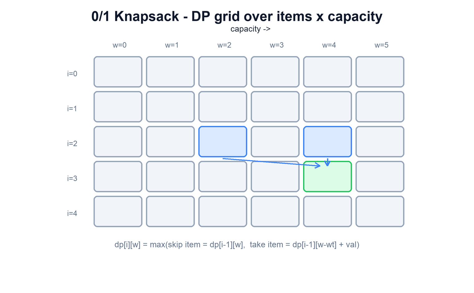
9. Greedy
A greedy algorithm builds a solution by repeatedly taking the choice that looks best right now; it is correct only when a local optimum provably leads to a global one.
Interval scheduling (activity selection)
To fit the most non-overlapping intervals, sort by finish time and keep each interval that starts after the last one taken.
function select_intervals(jobs):
  sort jobs by finish time ascending
  chosen = []
  last_end = -infinity
  for job in jobs:
    if job.start ≥ last_end:      # no overlap with last taken
      chosen.append(job)
      last_end = job.finish
  return chosen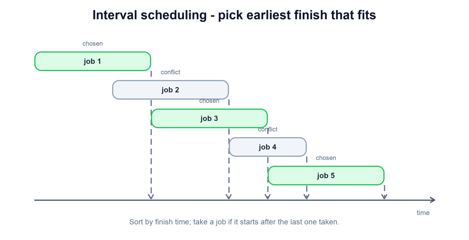
10. Divide & Conquer
Divide and conquer splits a problem into independent subproblems, solves each recursively, and combines the results — the split and combine steps define the algorithm.
Merge sort
Split the array to single elements (trivially sorted), then merge sorted halves back together in linear time per level.
function merge_sort(a):
  if len(a) ≤ 1: return a
  mid = len(a) / 2
  left  = merge_sort(a[:mid])
  right = merge_sort(a[mid:])
  return merge(left, right)         # combine two sorted runs

function merge(left, right):
  out = []
  while left and right:
    if left[0] ≤ right[0]: out.append(left.pop_front())
    else:                   out.append(right.pop_front())
  return out + left + right         # append leftovers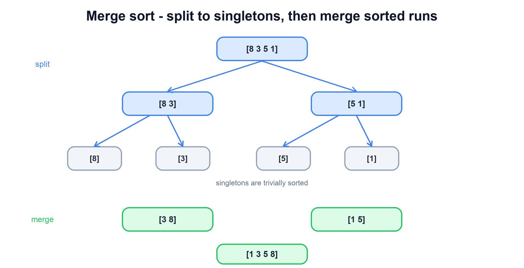
Quick sort
Pick a pivot, partition the array into elements smaller and larger than it, then recurse on each side; the pivot lands in its final place.
function quick_sort(a, lo, hi):
  if lo ≥ hi: return
  p = partition(a, lo, hi)          # pivot settles at index p
  quick_sort(a, lo, p-1)
  quick_sort(a, p+1, hi)

function partition(a, lo, hi):
  pivot = a[hi]
  i = lo
  for j from lo to hi-1:
    if a[j] < pivot:
      swap(a[i], a[j]); i = i + 1    # smaller items to the left
  swap(a[i], a[hi])
  return i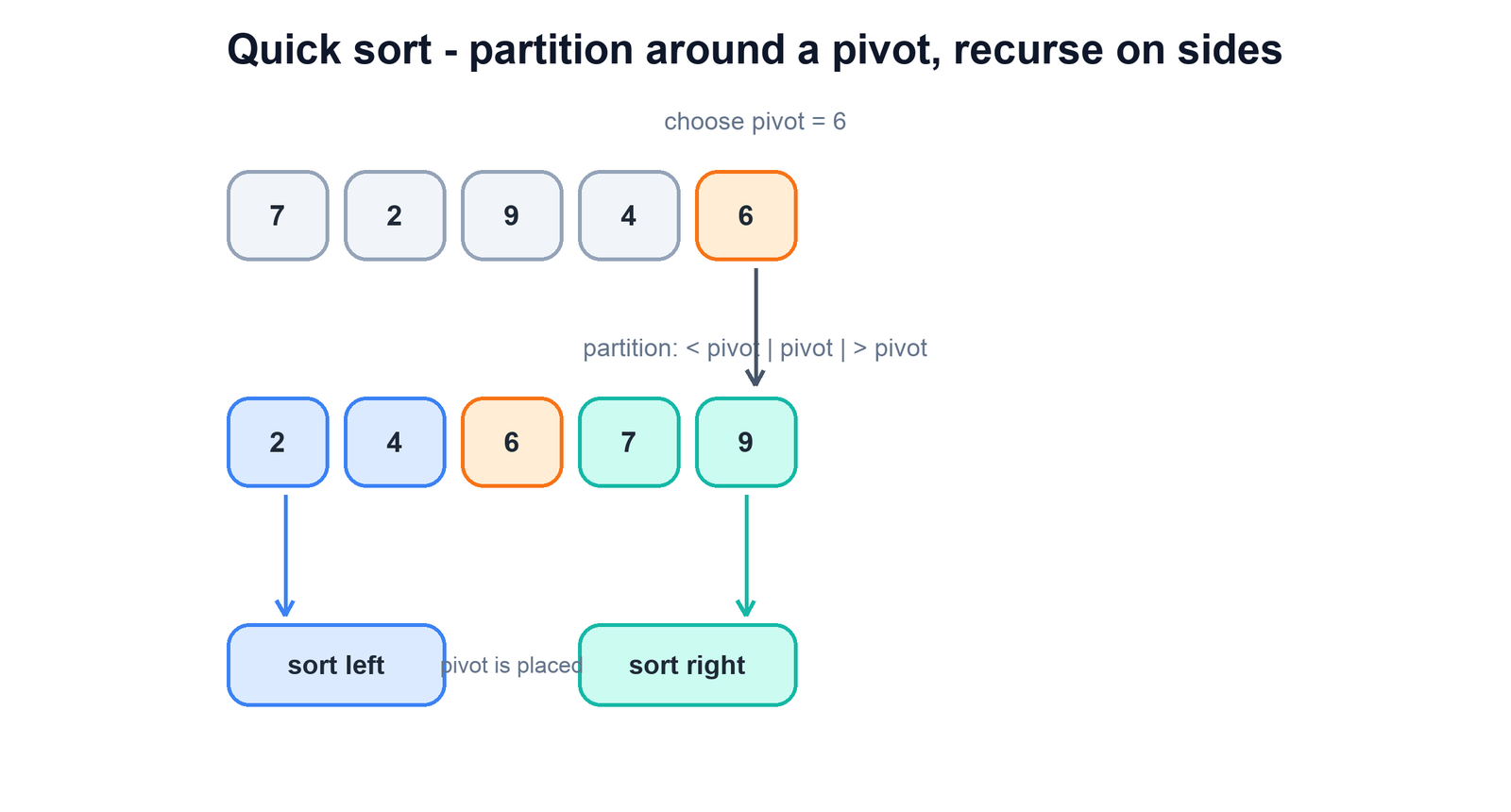
11. Heap / Top-K
A binary heap gives O(log n) access to the smallest or largest element, which makes it the natural structure for streaming top-K and running-median style problems.
Kth largest element
Keep a min-heap of size k; the root is the smallest of the k best seen, so any larger incoming value evicts it, leaving the kth largest at the root.
function kth_largest(stream, k):
  heap = min_heap()                 # size capped at k
  for value in stream:
    if len(heap) < k:
      heap.push(value)
    else if value > heap.peek():    # bigger than current kth
      heap.pop()
      heap.push(value)
  return heap.peek()                # root = kth largest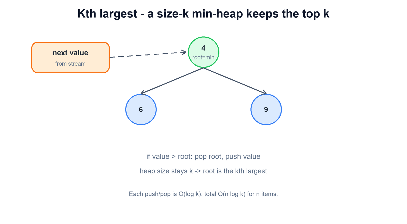
12. Union-Find (Disjoint Set)
Union-Find tracks a partition of elements into disjoint sets, supporting near-constant-time merge and same-set queries via path compression and union by rank.
Cycle detection / connected components
Each element points toward a root; two elements share a set when they share a root, and an edge whose endpoints already share a root closes a cycle.
function find(x):
  while parent[x] != x:
    parent[x] = parent[parent[x]]   # path compression
    x = parent[x]
  return x

function union(x, y):
  rx, ry = find(x), find(y)
  if rx == ry: return false         # already joined -> cycle
  if rank[rx] < rank[ry]: swap(rx, ry)
  parent[ry] = rx                   # attach smaller under larger
  if rank[rx] == rank[ry]: rank[rx] += 1
  return true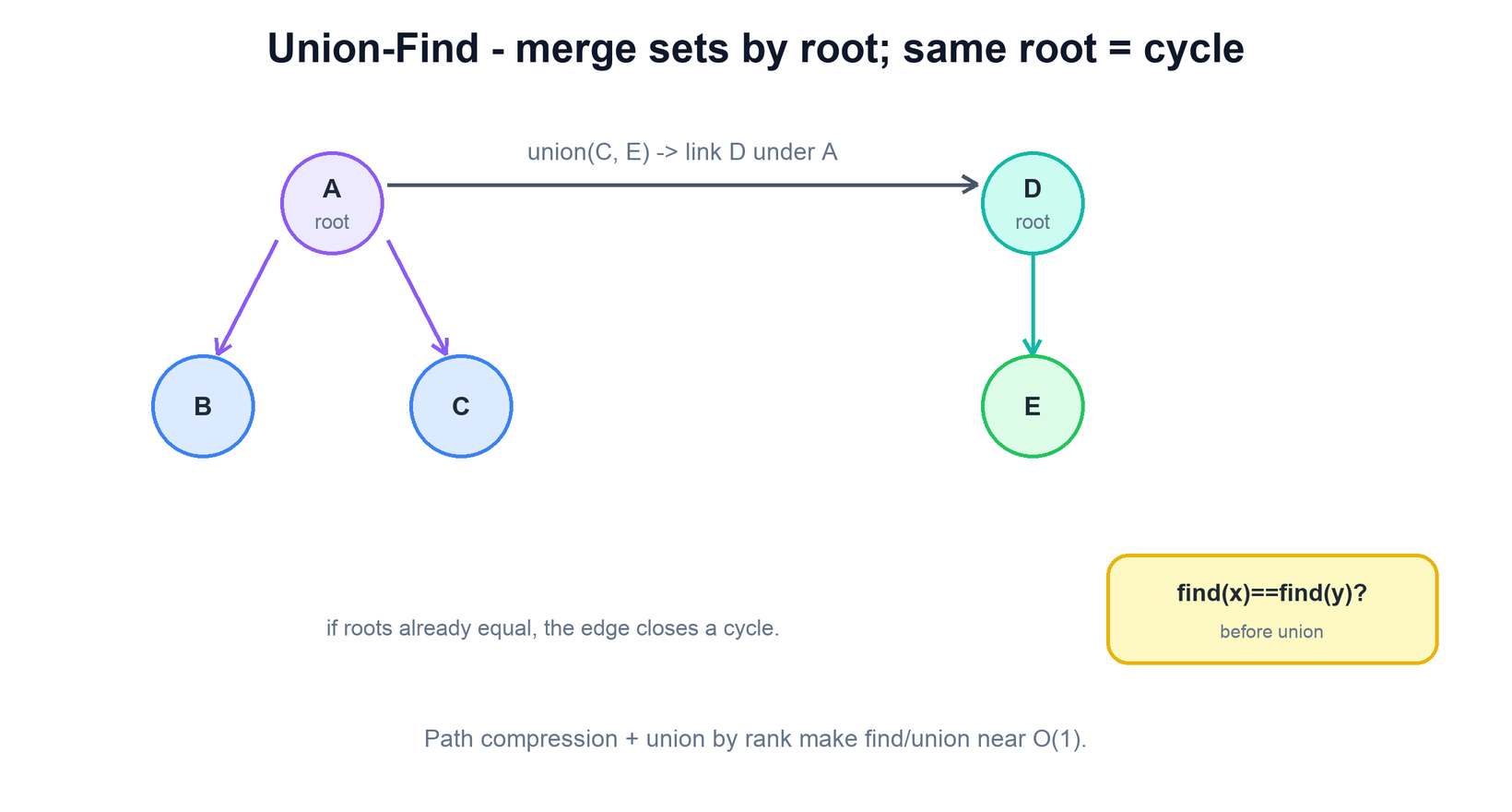
13. Topological Sort
A topological sort orders the nodes of a directed acyclic graph so every edge points forward — the standard way to sequence tasks with dependencies.
Kahn’s algorithm (course schedule)
Repeatedly take a node with no remaining prerequisites (in-degree 0) and remove it, decrementing its neighbors; if any node is left, a cycle exists.
function topo_sort(nodes, edges):
  compute in_degree[v] for all v
  queue = all v with in_degree[v] == 0
  order = []
  while queue not empty:
    u = queue.pop()
    order.append(u)
    for v in neighbors(u):
      in_degree[v] -= 1             # prerequisite satisfied
      if in_degree[v] == 0: queue.push(v)
  if len(order) < len(nodes): return CYCLE   # not a DAG
  return order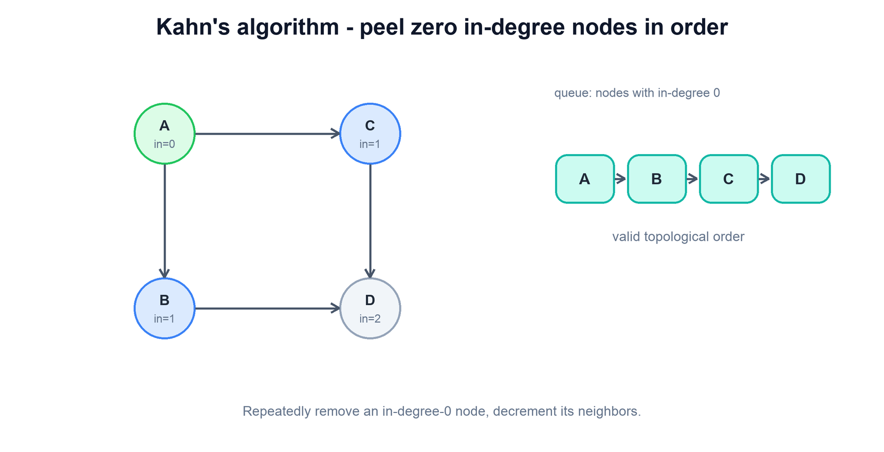
14. Graph Shortest Path — Dijkstra
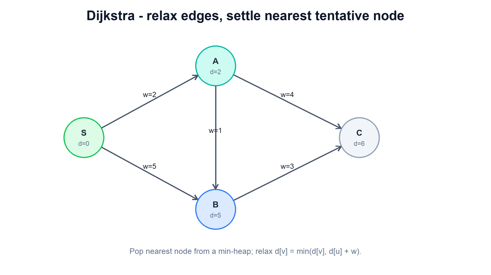
Dijkstra finds shortest paths from a source in a graph with non-negative edge weights by always settling the nearest unvisited node next.
Dijkstra’s algorithm
Keep tentative distances in a min-heap; pop the closest node, mark it final, and relax each outgoing edge to shorten its neighbors’ distances.
function dijkstra(graph, source):
  dist = map with default infinity
  dist[source] = 0
  heap = min_heap of (0, source)
  while heap not empty:
    d, u = heap.pop()               # nearest tentative node
    if d > dist[u]: continue        # stale entry, skip
    for (v, w) in graph[u]:
      if dist[u] + w < dist[v]:     # relax the edge
        dist[v] = dist[u] + w
        heap.push((dist[v], v))
  return dist